---
title: "mCAs"
subtitle: "Reproducing Key Concepts from Loh et al. (2018) & Terao (2026)"
author: "Computational Genomics Analysis"
date: today
format:
html:
toc: true
toc-depth: 3
theme: journal
code-fold: true
code-tools: true
number-sections: true
fig-cap-location: bottom
execute:
warning: false
message: false
bibliography: references.bib
---
## Introduction
Clonal haematopoiesis occurs when haematopoietic stem cells acquire somatic mutations that confer a survival advantage, leading to clonal expansion. This phenomenon is particularly prevalent in older individuals and is associated with increased risk of haematological malignancies, cardiovascular disease, and ageing-related phenotypes.
Loh et al. (2018) developed a landmark method for detecting **mosaic chromosomal alterations (mCAs)** from DNA microarray data, enabling large-scale population studies of clonal haematopoiesis without requiring expensive whole-exome or whole-genome sequencing.
This document walks through the core analytical concepts behind mCA detection, including B-allele frequency (BAF) deviation analysis, log2 R ratio (LRR) interpretation, and classification of mosaic events.
## Simulating Microarray Intensity Data
### Generating SNP probe data {#sec-snp-sim}
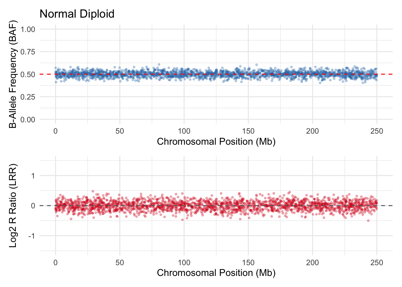
We begin by simulating microarray-like data for heterozygous SNPs across a chromosome, mimicking the signals used by the Loh et al. algorithm.
```{r}
#| label: simulate-snp-data
#| fig-cap: "Simulated BAF and LRR across a chromosome for a normal (non-mosaic) individual."
library(tidyverse)
library(patchwork)

set.seed(42)

n_snps <- 2000
positions <- sort(runif(n_snps, min = 0, max = 250)) # Mb along chromosome

# Normal diploid: BAF ~ 0.5, LRR ~ 0
simulate_normal <- function(n) {
 tibble(
   position = positions,
   BAF = rnorm(n, mean = 0.5, sd = 0.03),
   LRR = rnorm(n, mean = 0.0, sd = 0.15)
 )
}

normal_data <- simulate_normal(n_snps)

p_baf <- ggplot(normal_data, aes(position, BAF)) +
 geom_point(alpha = 0.3, size = 0.8, colour = "#2c7bb6") +
 geom_hline(yintercept = 0.5, linetype = "dashed", colour = "red") +
 labs(x = "Chromosomal Position (Mb)", y = "B-Allele Frequency (BAF)",
      title = "Normal Diploid") +
 ylim(0, 1) +
 theme_minimal(base_size = 12)

p_lrr <- ggplot(normal_data, aes(position, LRR)) +
 geom_point(alpha = 0.3, size = 0.8, colour = "#d7191c") +
 geom_hline(yintercept = 0, linetype = "dashed", colour = "grey40") +
 labs(x = "Chromosomal Position (Mb)", y = "Log2 R Ratio (LRR)") +
 ylim(-1.5, 1.5) +
 theme_minimal(base_size = 12)

p_baf / p_lrr
```
### Simulating a mosaic event
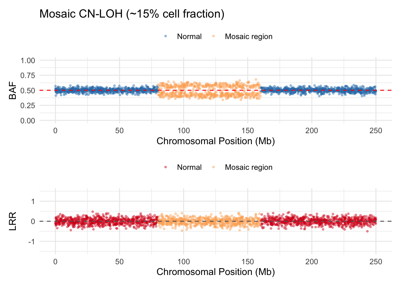
Now we introduce a mosaic chromosomal alteration — a region of copy-number neutral loss of heterozygosity (CN-LOH) affecting a fraction of cells. This shifts BAF away from 0.5 while LRR remains near zero.
```{r}
#| label: simulate-mosaic
#| fig-cap: "Simulated mCA: CN-LOH event between 80–160 Mb at ~15% cell fraction."
cell_fraction <- 0.15
mosaic_start <- 80
mosaic_end <- 160

simulate_mosaic_cnloh <- function(data, cf, start, end) {
 data |>
   mutate(
     in_mosaic = position >= start & position <= end,
     # CN-LOH shifts BAF towards 0 or 1 proportionally to cell fraction
     BAF_mosaic = if_else(
       in_mosaic,
       BAF + sample(c(-1, 1), n(), replace = TRUE) * cf * 0.5,
       BAF
     ),
     LRR_mosaic = LRR  # CN-LOH: no copy number change
   )
}

mosaic_data <- simulate_mosaic_cnloh(normal_data, cell_fraction,
                                      mosaic_start, mosaic_end)

p_baf_m <- ggplot(mosaic_data, aes(position, BAF_mosaic, colour = in_mosaic)) +
 geom_point(alpha = 0.4, size = 0.8) +
 geom_hline(yintercept = 0.5, linetype = "dashed", colour = "red") +
 scale_colour_manual(values = c("FALSE" = "#2c7bb6", "TRUE" = "#fdae61"),
                     labels = c("Normal", "Mosaic region")) +
 labs(x = "Chromosomal Position (Mb)", y = "BAF",
      title = "Mosaic CN-LOH (~15% cell fraction)", colour = NULL) +
 ylim(0, 1) +
 theme_minimal(base_size = 12) +
 theme(legend.position = "top")

p_lrr_m <- ggplot(mosaic_data, aes(position, LRR_mosaic, colour = in_mosaic)) +
 geom_point(alpha = 0.4, size = 0.8) +
 geom_hline(yintercept = 0, linetype = "dashed", colour = "grey40") +
 scale_colour_manual(values = c("FALSE" = "#d7191c", "TRUE" = "#fdae61"),
                     labels = c("Normal", "Mosaic region")) +
 labs(x = "Chromosomal Position (Mb)", y = "LRR", colour = NULL) +
 ylim(-1.5, 1.5) +
 theme_minimal(base_size = 12) +
 theme(legend.position = "top")

p_baf_m / p_lrr_m
```
## Detecting BAF Deviations
### Statistical framework for mCA detection
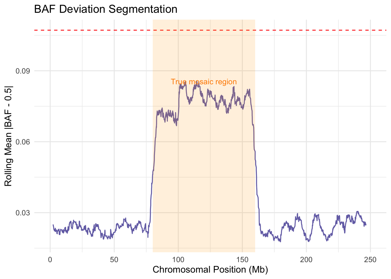
The core statistical insight is that heterozygous SNPs in a mosaic region show a consistent shift of BAF away from 0.5 towards one haplotype. We can test this with a segmentation approach.
```{r}
#| label: baf-deviation-test
#| fig-cap: "Rolling median of |BAF - 0.5| highlights the mosaic region."
window_size <- 50

mosaic_data <- mosaic_data |>
 arrange(position) |>
 mutate(
   baf_dev = abs(BAF_mosaic - 0.5),
   rolling_dev = zoo::rollmean(baf_dev, k = window_size,
                                fill = NA, align = "center")
 )

# Simple threshold-based detection
threshold <- mean(mosaic_data$baf_dev, na.rm = TRUE) +
 2 * sd(mosaic_data$baf_dev, na.rm = TRUE)

ggplot(mosaic_data, aes(position, rolling_dev)) +
 geom_line(colour = "#7570b3", linewidth = 0.6) +
 geom_hline(yintercept = threshold, linetype = "dashed",
            colour = "red", linewidth = 0.5) +
 annotate("rect", xmin = mosaic_start, xmax = mosaic_end,
          ymin = -Inf, ymax = Inf, alpha = 0.15, fill = "orange") +
 annotate("text", x = (mosaic_start + mosaic_end) / 2, y = max(mosaic_data$rolling_dev, na.rm = TRUE),
          label = "True mosaic region", size = 3.5, colour = "darkorange") +
 labs(x = "Chromosomal Position (Mb)",
      y = "Rolling Mean |BAF - 0.5|",
      title = "BAF Deviation Segmentation") +
 theme_minimal(base_size = 12)
```
## Classification of Mosaic Events
### Three classes of mCAs
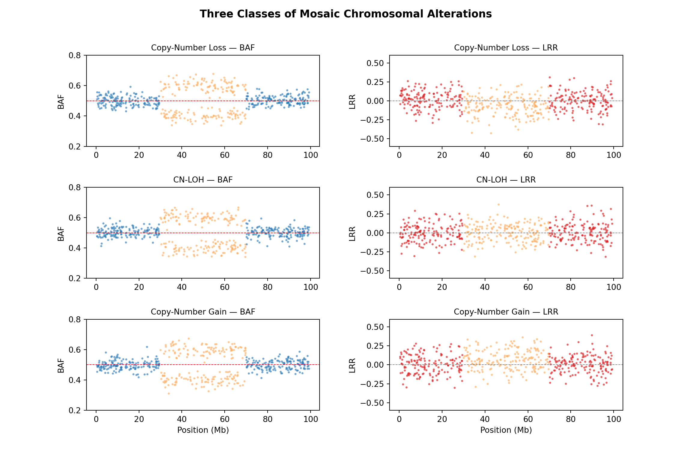
Mosaic events are classified into three categories based on the combination of BAF and LRR patterns:
| Class | BAF Pattern | LRR Pattern | Biological Interpretation |
|:-------|:---------------|:-----------------|:-------------------------------|
| Loss | Split from 0.5 | Decreased (\< 0) | Deletion of one copy |
| CN-LOH | Split from 0.5 | Near 0 | Duplication replacing one copy |
| Gain | Split from 0.5 | Increased (\> 0) | Gain of one copy |
```{python}
#| label: simulate-three-classes
#| fig-cap: "The three classes of mosaic chromosomal alterations with characteristic BAF/LRR signatures."
import numpy as np
import matplotlib.pyplot as plt
import matplotlib.gridspec as gridspec

np.random.seed(42)

n = 500
pos = np.sort(np.random.uniform(0, 100, n))
mosaic_mask = (pos > 30) & (pos < 70)
cell_frac = 0.20

fig = plt.figure(figsize=(12, 8))
gs = gridspec.GridSpec(3, 2, hspace=0.45, wspace=0.3)

classes = {
   "Copy-Number Loss": {"baf_shift": 0.5, "lrr_shift": -0.4},
   "CN-LOH": {"baf_shift": 0.5, "lrr_shift": 0.0},
   "Copy-Number Gain": {"baf_shift": 0.5, "lrr_shift": 0.3},
}

for i, (name, params) in enumerate(classes.items()):
   baf = np.random.normal(0.5, 0.03, n)
   lrr = np.random.normal(0.0, 0.12, n)

   direction = np.random.choice([-1, 1], n)
   baf[mosaic_mask] += direction[mosaic_mask] * cell_frac * params["baf_shift"]
   lrr[mosaic_mask] += cell_frac * params["lrr_shift"]

   colours_baf = np.where(mosaic_mask, "#fdae61", "#2c7bb6")
   colours_lrr = np.where(mosaic_mask, "#fdae61", "#d7191c")

   ax_baf = fig.add_subplot(gs[i, 0])
   ax_baf.scatter(pos, baf, c=colours_baf, s=3, alpha=0.5)
   ax_baf.axhline(0.5, ls="--", c="red", lw=0.7)
   ax_baf.set_ylim(0.2, 0.8)
   ax_baf.set_ylabel("BAF")
   ax_baf.set_title(f"{name} — BAF", fontsize=10)

   ax_lrr = fig.add_subplot(gs[i, 1])
   ax_lrr.scatter(pos, lrr, c=colours_lrr, s=3, alpha=0.5)
   ax_lrr.axhline(0.0, ls="--", c="grey", lw=0.7)
   ax_lrr.set_ylim(-0.6, 0.6)
   ax_lrr.set_ylabel("LRR")
   ax_lrr.set_title(f"{name} — LRR", fontsize=10)

   if i == 2:
       ax_baf.set_xlabel("Position (Mb)")
       ax_lrr.set_xlabel("Position (Mb)")

plt.suptitle("Three Classes of Mosaic Chromosomal Alterations",
            fontsize=13, fontweight="bold", y=0.98)
plt.savefig("mca_classes.png", dpi=150, bbox_inches="tight")
plt.show()
```
## Age-Associated Prevalence
### Modelling mCA prevalence by age
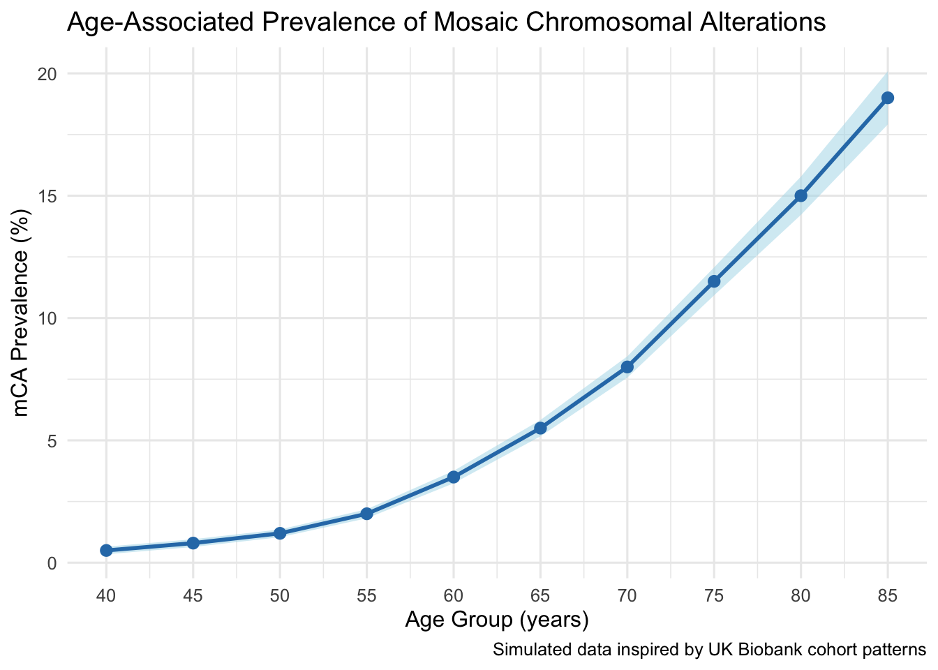
Clonal haematopoiesis increases sharply with age. We model the expected prevalence based on patterns reported in the UK Biobank analysis.
```{r}
#| label: age-prevalence
#| fig-cap: "Simulated mCA prevalence by age group, consistent with population cohort findings."
# Approximate prevalence data inspired by UK Biobank findings
age_data <- tibble(
 age_group = seq(40, 85, by = 5),
 prevalence_pct = c(0.5, 0.8, 1.2, 2.0, 3.5, 5.5, 8.0, 11.5, 15.0, 19.0),
 n_individuals = c(8000, 12000, 18000, 22000, 20000, 18000, 15000, 12000, 8000, 5000)
)

age_data <- age_data |>
 mutate(
   se = sqrt(prevalence_pct * (100 - prevalence_pct) / n_individuals),
   lower = prevalence_pct - 1.96 * se,
   upper = prevalence_pct + 1.96 * se
 )

ggplot(age_data, aes(age_group, prevalence_pct)) +
 geom_ribbon(aes(ymin = lower, ymax = upper), fill = "#abd9e9", alpha = 0.5) +
 geom_line(colour = "#2c7bb6", linewidth = 1) +
 geom_point(colour = "#2c7bb6", size = 2.5) +
 scale_x_continuous(breaks = seq(40, 85, 5)) +
 labs(
   x = "Age Group (years)",
   y = "mCA Prevalence (%)",
   title = "Age-Associated Prevalence of Mosaic Chromosomal Alterations",
   caption = "Simulated data inspired by UK Biobank cohort patterns"
 ) +
 theme_minimal(base_size = 12)
```
## Sensitivity vs. Cell Fraction
### Detection power by mosaic cell fraction
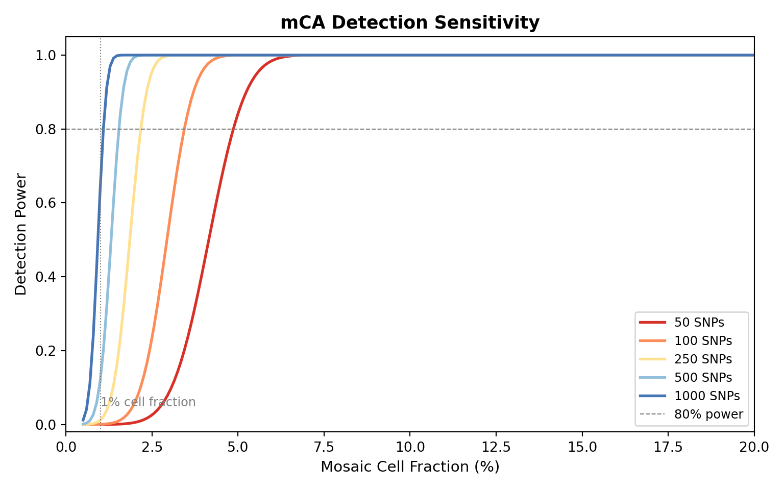
A remarkable feature of the Loh et al. algorithm is its ability to detect events present in as few as \~1% of cells. We model detection sensitivity as a function of cell fraction and number of informative SNPs.
```{python}
#| label: sensitivity-model
#| fig-cap: "Estimated detection power as a function of mosaic cell fraction and SNP density in the affected region."
import numpy as np
import matplotlib.pyplot as plt
from scipy.stats import norm

def detection_power(cell_fraction, n_snps, noise_sd=0.03, alpha=1e-6):
   """
   Approximate detection power for mCA detection.

   The signal is the mean BAF deviation (cell_fraction * 0.5) across
   n_snps heterozygous SNPs. Under the null, BAF deviations are
   noise ~ N(0, noise_sd / sqrt(n_snps)).
   """
   signal = cell_fraction * 0.5
   se = noise_sd / np.sqrt(n_snps)
   z_crit = norm.ppf(1 - alpha / 2)
   power = 1 - norm.cdf(z_crit - signal / se) + norm.cdf(-z_crit - signal / se)
   return power

cell_fractions = np.linspace(0.005, 0.20, 200)
snp_counts = [50, 100, 250, 500, 1000]
colours = ["#d73027", "#fc8d59", "#fee090", "#91bfdb", "#4575b4"]

fig, ax = plt.subplots(figsize=(8, 5))

for n_snps, col in zip(snp_counts, colours):
   power = [detection_power(cf, n_snps) for cf in cell_fractions]
   ax.plot(cell_fractions * 100, power, label=f"{n_snps} SNPs",
           color=col, linewidth=2)

ax.axhline(0.8, ls="--", color="grey", lw=0.8, label="80% power")
ax.axvline(1.0, ls=":", color="grey", lw=0.8)
ax.annotate("1% cell fraction", xy=(1.0, 0.05), fontsize=9, color="grey")
ax.set_xlabel("Mosaic Cell Fraction (%)", fontsize=11)
ax.set_ylabel("Detection Power", fontsize=11)
ax.set_title("mCA Detection Sensitivity", fontsize=13, fontweight="bold")
ax.legend(loc="lower right", fontsize=9)
ax.set_ylim(-0.02, 1.05)
ax.set_xlim(0, 20)
plt.tight_layout()
plt.savefig("sensitivity.png", dpi=150, bbox_inches="tight")
plt.show()
```
## Germline–Somatic Interaction
### Association between germline variants and mCA risk
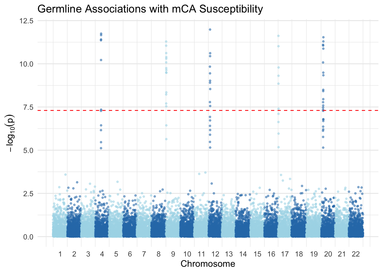
Loh et al. found that specific germline variants increase the risk of acquiring mCAs. We simulate a simple GWAS-like analysis of germline variant associations.
```{r}
#| label: germline-association
#| fig-cap: "Simulated Manhattan plot for germline variants associated with mCA susceptibility."
library(tidyverse)

set.seed(123)

n_variants <- 20000
n_chr <- 22

gwas_data <- tibble(
 chr = sample(1:n_chr, n_variants, replace = TRUE),
 pos = runif(n_variants, 1e6, 2.5e8),
 p_value = runif(n_variants)
)

# Inject signals on specific chromosomes (inspired by reported loci)
signal_loci <- tribble(
 ~chr, ~pos,       ~gene,
 4,    106e6,      "TET2",
 9,    5.0e6,      "JAK2",
 12,   25.4e6,     "KRAS",
 17,   7.6e6,      "TP53",
 20,   32.3e6,     "DNMT3A"
)

for (i in seq_len(nrow(signal_loci))) {
 nearby <- which(
   gwas_data$chr == signal_loci$chr[i] &
   abs(gwas_data$pos - signal_loci$pos[i]) < 2e6
 )
 if (length(nearby) > 0) {
   gwas_data$p_value[nearby] <- 10^(-runif(length(nearby), 5, 12))
 }
}

gwas_data <- gwas_data |>
 mutate(log_p = -log10(p_value)) |>
 arrange(chr, pos) |>
 mutate(index = row_number())

chr_midpoints <- gwas_data |>
 group_by(chr) |>
 summarise(mid = mean(index), .groups = "drop")

ggplot(gwas_data, aes(index, log_p, colour = factor(chr %% 2))) +
 geom_point(alpha = 0.5, size = 0.8) +
 geom_hline(yintercept = -log10(5e-8), linetype = "dashed",
            colour = "red", linewidth = 0.5) +
 scale_colour_manual(values = c("#2c7bb6", "#abd9e9")) +
 scale_x_continuous(breaks = chr_midpoints$mid,
                    labels = chr_midpoints$chr) +
 labs(x = "Chromosome", y = expression(-log[10](p)),
      title = "Germline Associations with mCA Susceptibility") +
 theme_minimal(base_size = 12) +
 theme(legend.position = "none",
       panel.grid.major.x = element_blank())
```
## CLL Risk Prediction
### Mosaic status improves leukaemia prediction
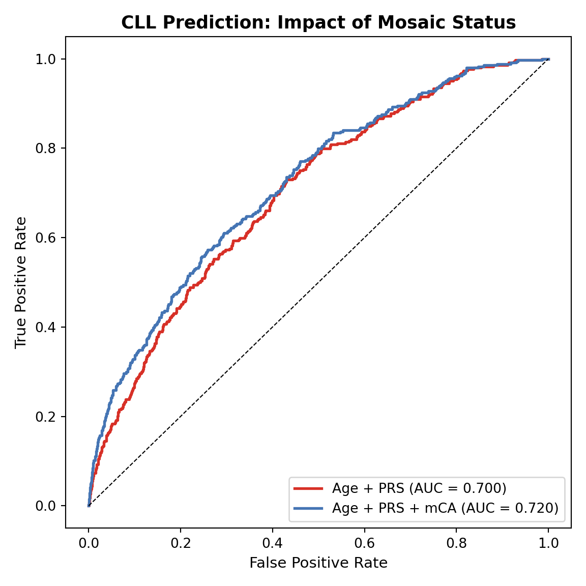
A key clinical finding was that incorporating mCA status significantly improved prediction of chronic lymphocytic leukaemia (CLL). We demonstrate this concept by comparing ROC curves from models with and without mosaic features.
```{python}
#| label: cll-prediction
#| fig-cap: "ROC curves comparing CLL prediction with and without mCA status as a feature."
import numpy as np
import matplotlib.pyplot as plt
from sklearn.linear_model import LogisticRegression
from sklearn.metrics import roc_curve, auc

np.random.seed(42)
n = 5000

# Simulate features
age = np.random.normal(65, 10, n)
prs = np.random.normal(0, 1, n)  # polygenic risk score
mca_status = np.random.binomial(1, 0.06, n)  # ~6% prevalence

# Simulate CLL outcome
logit_base = -5 + 0.03 * age + 0.8 * prs
logit_full = logit_base + 1.5 * mca_status  # mCA is a strong predictor
prob_cll = 1 / (1 + np.exp(-logit_full))
cll = np.random.binomial(1, prob_cll)

# Model without mCA
X_base = np.column_stack([age, prs])
model_base = LogisticRegression(max_iter=1000).fit(X_base, cll)
pred_base = model_base.predict_proba(X_base)[:, 1]

# Model with mCA
X_full = np.column_stack([age, prs, mca_status])
model_full = LogisticRegression(max_iter=1000).fit(X_full, cll)
pred_full = model_full.predict_proba(X_full)[:, 1]

fpr_b, tpr_b, _ = roc_curve(cll, pred_base)
fpr_f, tpr_f, _ = roc_curve(cll, pred_full)
auc_b = auc(fpr_b, tpr_b)
auc_f = auc(fpr_f, tpr_f)

fig, ax = plt.subplots(figsize=(6, 6))
ax.plot(fpr_b, tpr_b, color="#d73027", lw=2, label=f"Age + PRS (AUC = {auc_b:.3f})")
ax.plot(fpr_f, tpr_f, color="#4575b4", lw=2, label=f"Age + PRS + mCA (AUC = {auc_f:.3f})")
ax.plot([0, 1], [0, 1], "k--", lw=0.8)
ax.set_xlabel("False Positive Rate", fontsize=11)
ax.set_ylabel("True Positive Rate", fontsize=11)
ax.set_title("CLL Prediction: Impact of Mosaic Status", fontsize=13, fontweight="bold")
ax.legend(loc="lower right", fontsize=10)
plt.tight_layout()
plt.savefig("cll_roc.png", dpi=150, bbox_inches="tight")
plt.show()
```
## MoChA Pipeline Overview
The detection algorithm was packaged into **MoChA** (Mosaic Chromosomal Alterations), a user-friendly pipeline. Below is an overview of the workflow:
```{r}
#| label: mocha-workflow
#| fig-cap: "Schematic workflow of the MoChA analysis pipeline."
library(DiagrammeR)

grViz("
digraph mocha_pipeline {
 graph [rankdir=TB, fontname='Helvetica', bgcolor='transparent']
 node  [shape=box, style='filled,rounded', fontname='Helvetica',
        fontsize=11, fillcolor='#e0f3f8', color='#4575b4', penwidth=1.5]
 edge  [color='#4575b4', penwidth=1.2]

 A [label='Raw Microarray\\nIntensity Data (.idat)']
 B [label='Genotype Calling\\n& QC']
 C [label='Extract BAF & LRR\\nfor Het SNPs']
 D [label='Denoising &\\nSignal Correction']
 E [label='Long-Range\\nHaplotype Phasing']
 F [label='Mosaic Event\\nDetection (HMM)']
 G [label='Classification:\\nLoss / CN-LOH / Gain']
 H [label='Cell Fraction\\nEstimation']
 I [label='Output: mCA\\nCall Set', fillcolor='#fdae61']

 A -> B -> C -> D -> E -> F -> G -> H -> I
}
")
```
## Summary
This document demonstrated the core analytical concepts behind mCA detection from microarray data:
- **BAF deviation analysis** identifies allelic imbalance in mosaic regions
- **LRR patterns** distinguish loss, CN-LOH, and gain events
- **Statistical power** depends on cell fraction and SNP density, with detection possible at cell fractions as low as \~1%
- **Germline–somatic interactions** reveal inherited predisposition to clonal expansion
- **Clinical utility** is demonstrated by improved CLL risk prediction when incorporating mCA status
The MoChA software makes this analysis accessible to researchers with standard microarray datasets.
## References
Loh, P.-R. et al. Insights into clonal haematopoiesis from 8,342 mosaic chromosomal alterations. *Nature* **559**, 350–355 (2018).
Terao, C. From DNA microarrays to somatic mosaicism in population cohorts. *Nature Reviews Genetics* (2026).
## Session Info
```{r}
#| label: session-info
sessionInfo()
```