---
title: "The Fitness, Fate, and Function of Clonal Hematopoiesis"
subtitle: "A Comprehensive Reference Guide"
author: "Yash Pershad"
date: today
format:
html:
toc: true
toc-depth: 4
toc-location: right
number-sections: true
code-fold: true
code-tools: true
theme: journal
highlight-style: github
fig-width: 8
fig-height: 6
execute:
warning: false
message: false
bibliography: references.bib
csl: https://raw.githubusercontent.com/citation-style-language/styles/master/nature.csl
---
# Somatic Mosaicism {#sec-mosaicism}
Somatic mosaicism refers to the occurrence of genetically distinct cell populations within a single individual, arising from postzygotic mutations that accumulate throughout life [@Yizhak2019]. Every cell acquires unique genetic changes — from single-nucleotide variants and small insertions/deletions to structural rearrangements and chromosomal aberrations — beginning with the first cell division after fertilization and continuing through aging.
The conceptual roots of somatic mosaicism trace back to Theodor Boveri's proposal that neoplasia could arise from a single cell acquiring a genetic change. Key milestones include Barbara McClintock's discovery of somatic transposition, Knudson's two-hit model of cancer (1971), and the discovery of somatic gene rearrangement in immune cells in the 1970s. The first human mosaic chromosomal abnormality was reported in 1960, and cytogenetic methods remained the primary detection tool until array-based and next-generation sequencing technologies dramatically improved sensitivity.
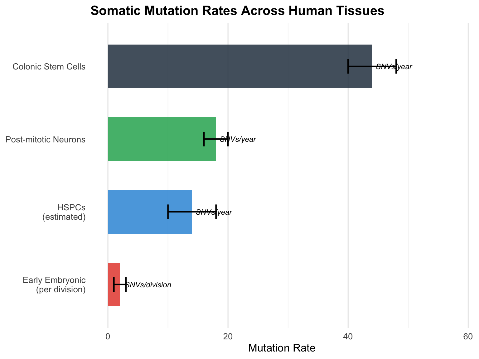
Somatic mutations accumulate at tissue-specific rates shaped by cell division frequency, environmental exposures, and intrinsic mutagenic processes. The **Somatic Mosaicism across Human Tissues (SMaHT) Network**, an NIH Common Fund initiative, aims to generate a reference catalog of somatic mutations across 19 tissue sites from 150 non-diseased donors.
## Tissue-Specific Somatic Mutation Rates
```{r}
#| label: fig-mutation-rates
#| fig-cap: "Estimated somatic mutation rates across human tissues. Post-mitotic neurons accumulate ~16-20 SNVs/year, while colonic stem cells accrue ~44/year."
library(ggplot2)

mutation_data <- data.frame(
  tissue = c("Post-mitotic Neurons", "Colonic Stem Cells",
             "Early Embryonic\n(per division)", "HSPCs\n(estimated)"),
  rate = c(18, 44, 2, 14),
  rate_low = c(16, 40, 1, 10),
  rate_high = c(20, 48, 3, 18),
  unit = c("SNVs/year", "SNVs/year", "SNVs/division", "SNVs/year")
)

ggplot(mutation_data, aes(x = reorder(tissue, rate), y = rate, fill = tissue)) +
  geom_col(alpha = 0.85, width = 0.6) +
  geom_errorbar(aes(ymin = rate_low, ymax = rate_high), width = 0.2, linewidth = 0.8) +
  geom_text(aes(label = unit), hjust = -0.1, size = 3.2, fontface = "italic") +
  coord_flip() +
  scale_fill_manual(values = c("#2C3E50", "#E74C3C", "#3498DB", "#27AE60")) +
  labs(
    x = NULL,
    y = "Mutation Rate",
    title = "Somatic Mutation Rates Across Human Tissues"
  ) +
  theme_minimal(base_size = 13) +
  theme(
    legend.position = "none",
    panel.grid.major.y = element_blank(),
    plot.title = element_text(face = "bold")
  ) +
  ylim(0, 58)
```
# Clonal Hematopoiesis {#sec-ch}
## Definition and Forms of Clonal Hematopoiesis
### Clonal Hematopoiesis of Indeterminate Potential (CHIP)
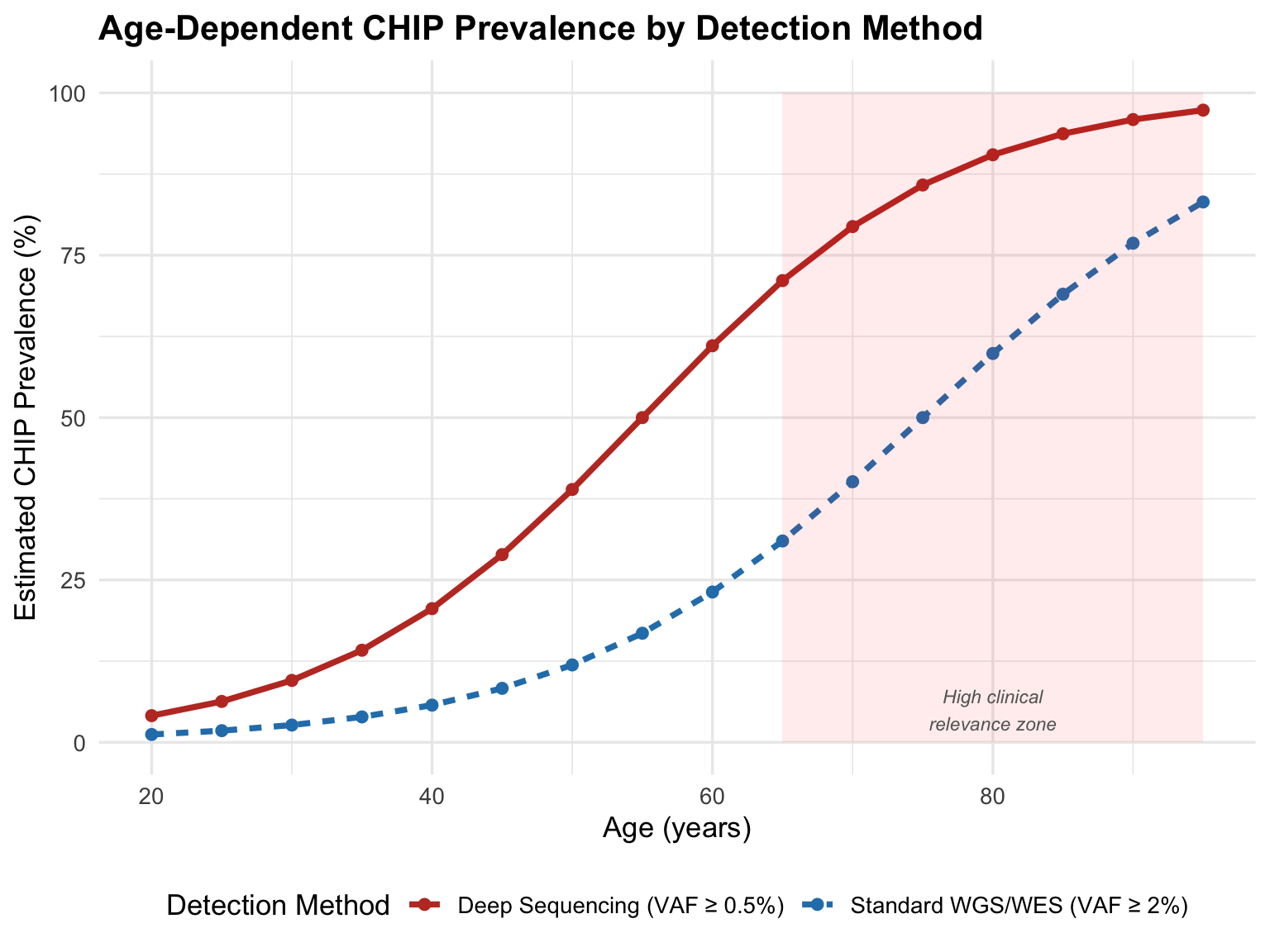
Clonal hematopoiesis of indeterminate potential (CHIP) is defined by the presence of a somatic mutation in a known leukemia-associated driver gene in the peripheral blood or bone marrow at a variant allele fraction (VAF) ≥ 2%, in the absence of a hematologic malignancy or unexplained cytopenia [@Jaiswal2014; @Genovese2014]. CHIP is predominantly an age-related phenomenon: prevalence is \<1% in individuals under 40, rises to \~10-20% by age 70, and may exceed 50-75% by age 90 when assessed with deep sequencing.
The most commonly mutated genes in CHIP are *DNMT3A*, *TET2*, and *ASXL1*, which together account for \~80% of detected clones. Although CHIP is classically defined by mutations in the \~75 canonical driver genes, in principle any mutation that produces a clonal expansion in the peripheral blood is a form of clonal hematopoiesis. Germline hereditary cancer syndromes (e.g., RUNX1-Familial Platelet Disorder) and telomere biology disorders may have unique drivers in the setting of differing selection pressures.
```{r}
#| label: fig-chip-prevalence
#| fig-cap: "Age-dependent prevalence of CHIP at standard WGS/WES detection thresholds versus deep sequencing approaches."
library(ggplot2)

age_seq <- seq(20, 95, by = 5)

standard <- 100 / (1 + exp(-0.08 * (age_seq - 75)))
deep_seq <- 100 / (1 + exp(-0.09 * (age_seq - 55)))

prev_data <- data.frame(
  Age = rep(age_seq, 2),
  Prevalence = c(standard, deep_seq),
  Method = rep(c("Standard WGS/WES (VAF ≥ 2%)", "Deep Sequencing (VAF ≥ 0.5%)"),
               each = length(age_seq))
)

ggplot(prev_data, aes(x = Age, y = Prevalence, color = Method, linetype = Method)) +
  geom_line(linewidth = 1.3) +
  geom_point(size = 2) +
  scale_color_manual(values = c("#C0392B", "#2980B9")) +
  labs(
    x = "Age (years)",
    y = "Estimated CHIP Prevalence (%)",
    title = "Age-Dependent CHIP Prevalence by Detection Method",
    color = "Detection Method",
    linetype = "Detection Method"
  ) +
  theme_minimal(base_size = 13) +
  theme(
    legend.position = "bottom",
    plot.title = element_text(face = "bold")
  ) +
  annotate("rect", xmin = 65, xmax = 95, ymin = 0, ymax = 100,
           alpha = 0.08, fill = "red") +
  annotate("text", x = 80, y = 5, label = "High clinical\nrelevance zone",
           size = 3, color = "grey40", fontface = "italic")
```
### Mosaic Chromosomal Alterations (mCAs)
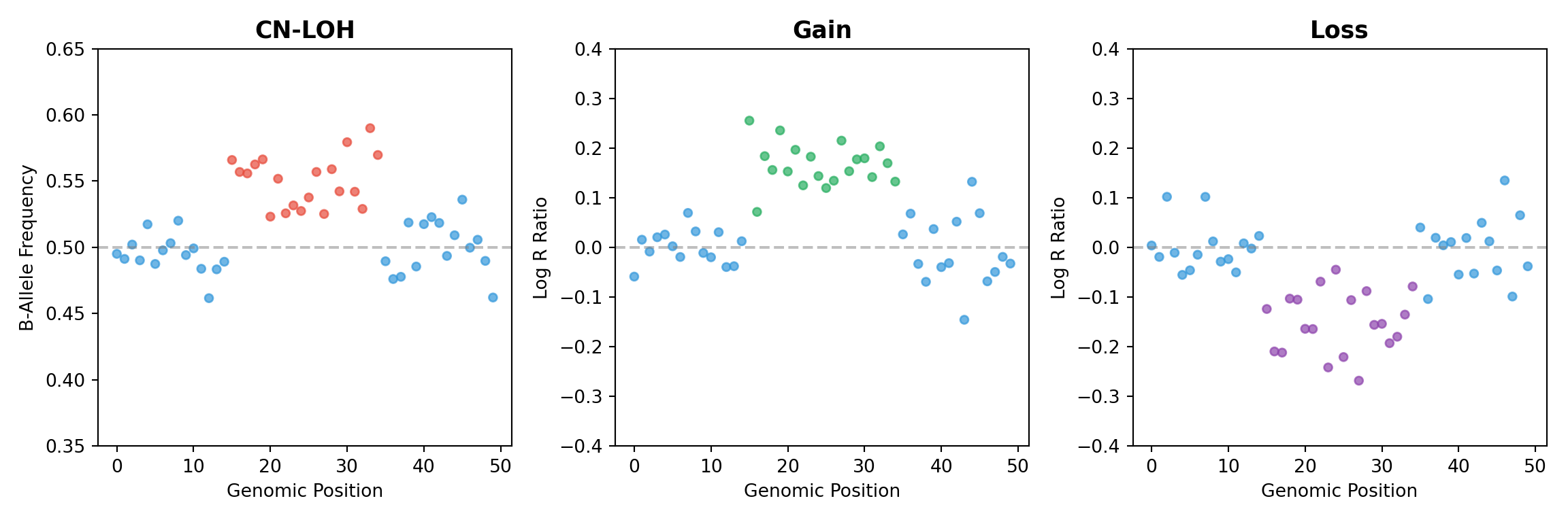
In contrast to CHIP, when large genomic regions (≥ 1 megabase) are affected, this is termed a mosaic chromosomal alteration (mCA). mCAs commonly affect the Y chromosome in males (mLOY) and the X chromosome in females (mLOX), but also involve autosomes [@Liu2024mca]. mCAs may involve gain, loss, or copy-neutral loss of heterozygosity (CN-LOH). Unlike CHIP which tends toward myeloid neoplasms, mCAs are often found in lymphoid neoplasms and cause a lymphoid bias in HSPC differentiation [@Pershad2024mca].
```{python}
#| label: fig-mca-types
#| fig-cap: "Overview of mosaic chromosomal alteration types and their detection signals."
import matplotlib.pyplot as plt
import matplotlib.patches as mpatches
import numpy as np

fig, axes = plt.subplots(1, 3, figsize=(12, 4))

# CN-LOH
ax = axes[0]
ax.set_title("CN-LOH", fontsize=13, fontweight='bold')
x = np.arange(50)
normal_baf = np.random.normal(0.5, 0.02, 50)
mosaic_baf = np.random.normal(0.5, 0.02, 50)
mosaic_baf[15:35] = np.random.normal(0.55, 0.02, 20)
ax.scatter(x, mosaic_baf, c=['#3498DB' if i < 15 or i >= 35 else '#E74C3C' for i in range(50)],
           s=20, alpha=0.7)
ax.set_ylabel("B-Allele Frequency")
ax.set_xlabel("Genomic Position")
ax.axhline(y=0.5, color='grey', linestyle='--', alpha=0.5)
ax.set_ylim(0.35, 0.65)
# Gain
ax = axes[1]
ax.set_title("Gain", fontsize=13, fontweight='bold')
lrr_normal = np.random.normal(0, 0.05, 50)
lrr_normal[15:35] = np.random.normal(0.15, 0.05, 20)
ax.scatter(x, lrr_normal, c=['#3498DB' if i < 15 or i >= 35 else '#27AE60' for i in range(50)],
           s=20, alpha=0.7)
ax.set_ylabel("Log R Ratio")
ax.set_xlabel("Genomic Position")
ax.axhline(y=0, color='grey', linestyle='--', alpha=0.5)
ax.set_ylim(-0.4, 0.4)
# Loss
ax = axes[2]
ax.set_title("Loss", fontsize=13, fontweight='bold')
lrr_loss = np.random.normal(0, 0.05, 50)
lrr_loss[15:35] = np.random.normal(-0.15, 0.05, 20)
ax.scatter(x, lrr_loss, c=['#3498DB' if i < 15 or i >= 35 else '#8E44AD' for i in range(50)],
           s=20, alpha=0.7)
ax.set_ylabel("Log R Ratio")
ax.set_xlabel("Genomic Position")
ax.axhline(y=0, color='grey', linestyle='--', alpha=0.5)
ax.set_ylim(-0.4, 0.4)
plt.tight_layout()
plt.savefig("mca_types.png", dpi=150, bbox_inches='tight')
plt.show()
```
## Detection of Clonal Hematopoiesis {#sec-detection}
### Sensitivity Limits of Population-Scale Sequencing
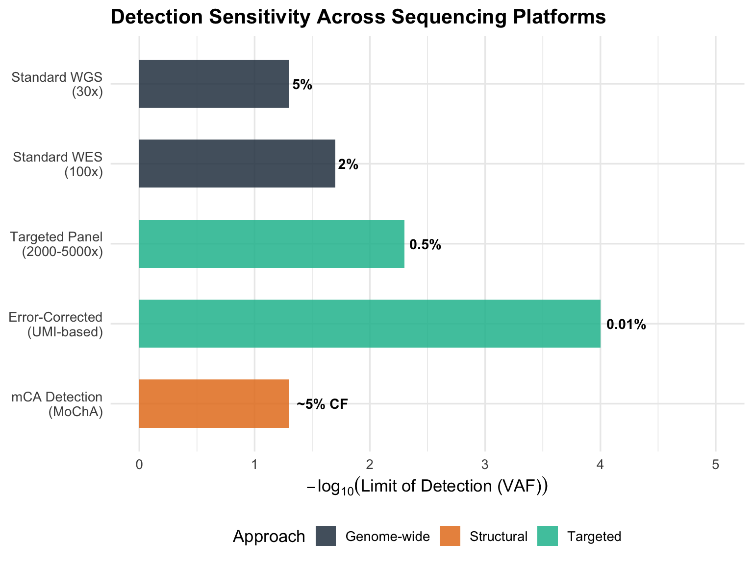
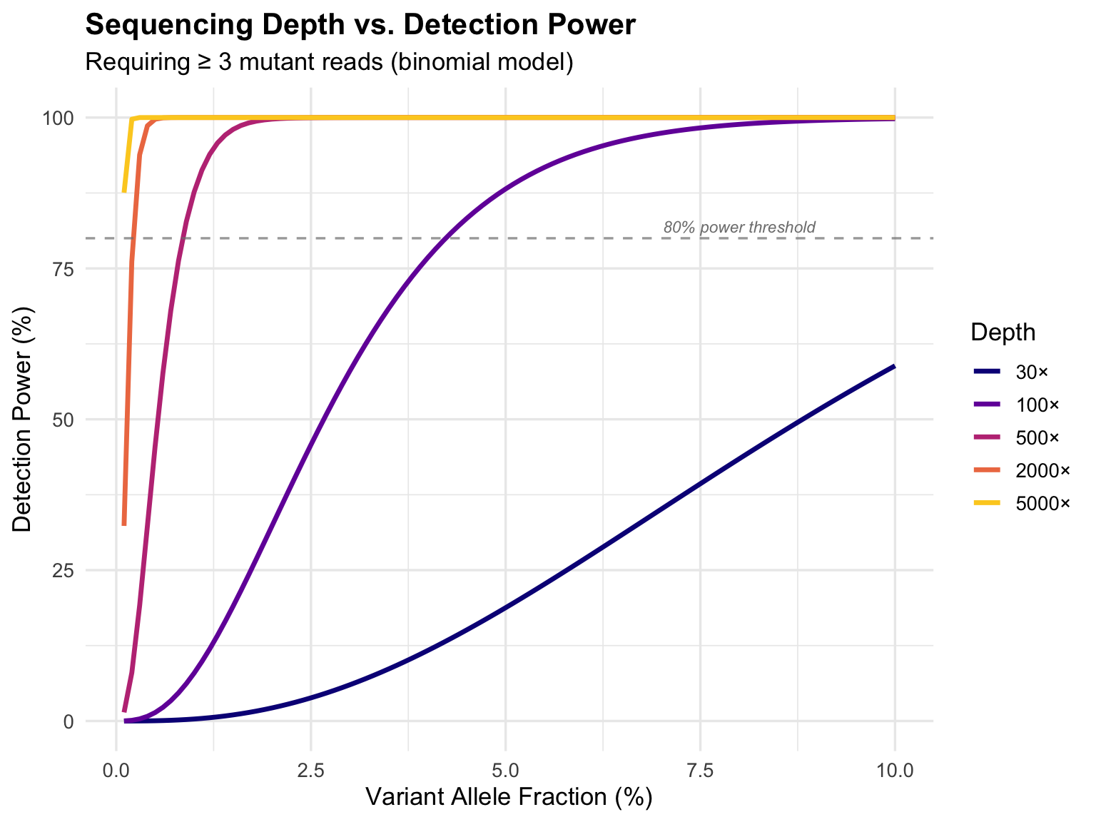
Standard WGS protocols achieve 30–50× coverage. At this depth, detecting a variant at 5% VAF results in only 1.5–2.5 mutant reads, making it statistically underpowered to distinguish true low-frequency somatic variants from stochastic sequencing errors [@Corty2025]. This detection threshold creates a significant **ascertainment bias**: 30× WGS misses the "micro-CH" landscape (VAF \< 0.02) which characterizes the majority of the population.
### Deep, Error-Corrected, Targeted Sequencing Approaches
Targeted sequencing panels achieve depths of 2,000–5,000× and lower the limit of detection to VAFs of 0.005 or below. Error-corrected sequencing utilizes **Unique Molecular Identifiers (UMIs)** to barcode original DNA molecules before amplification, enabling detection of "micro-CH" clones at VAFs as low as 10^-4^ or 10^-5^ [@Mack2024].
### Detection of Mosaic Chromosomal Alterations
mCA detection relies on analysis of common heterozygous germline variants. The primary detection signals include the **log R ratio** (total copy number) and the **B-allele frequency** (relative allele proportion). Modern pipelines use long-range phasing algorithms (e.g., Eagle2 or SHAPEIT4) with the MoChA tool to detect mosaicism at cell fractions as low as \~5% [@Loh2018; @Pershad2024mca].
```{r}
#| label: fig-detection-comparison
#| fig-cap: "Comparison of detection sensitivity across sequencing approaches for clonal hematopoiesis."
library(ggplot2)

detection <- data.frame(
  method = c("Standard WGS\n(30x)", "Standard WES\n(100x)",
             "Targeted Panel\n(2000-5000x)", "Error-Corrected\n(UMI-based)",
             "mCA Detection\n(MoChA)"),
  lod_vaf = c(0.05, 0.02, 0.005, 0.0001, 0.05),
  lod_label = c("5%", "2%", "0.5%", "0.01%", "~5% CF"),
  category = c("Genome-wide", "Genome-wide", "Targeted", "Targeted", "Structural")
)

detection$method <- factor(detection$method, levels = rev(detection$method))

ggplot(detection, aes(x = method, y = -log10(lod_vaf), fill = category)) +
  geom_col(alpha = 0.85, width = 0.6) +
  geom_text(aes(label = lod_label), hjust = -0.15, size = 3.8, fontface = "bold") +
  coord_flip() +
  scale_fill_manual(values = c("#2C3E50", "#E67E22", "#1ABC9C")) +
  labs(
    x = NULL,
    y = expression(-log[10]("Limit of Detection (VAF)")),
    title = "Detection Sensitivity Across Sequencing Platforms",
    fill = "Approach"
  ) +
  theme_minimal(base_size = 13) +
  theme(
    plot.title = element_text(face = "bold"),
    legend.position = "bottom"
  ) +
  ylim(0, 5)
```
## Clinical Significance of Clonal Hematopoiesis {#sec-clinical}
### Hematologic Consequences
The most direct consequence of CH is progression to hematologic malignancy. CHIP carriers face an approximately **7-fold increased risk** of hematologic malignancy [@Jaiswal2014]. However, absolute progression remains low — roughly 0.5–1% per year — meaning the majority of carriers will never develop an overt malignancy.
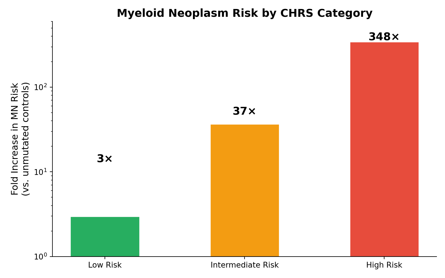
Risk stratification tools include the **Clonal Hematopoiesis Risk Score (CHRS)** and **Myeloid Neoplasm Predict (MNPredict)**, with NCCN guidelines stratifying myeloid neoplasm risk as 3-fold, 37-fold, and 348-fold in low-, intermediate-, and high-risk categories respectively [@Greenberg2025].
When CHIP occurs with unexplained persistent cytopenias (≥ 4 months), it is termed **clonal cytopenia of uncertain significance (CCUS)**, carrying dramatically higher progression risk. For mCAs, specific chromosomal arm alterations (6q, 11q, 13q, 17p, gain of chromosome 12) are highly specific (\>99%) for monoclonal B cell lymphocytosis and chronic lymphocytic leukemia.
```{python}
#| label: fig-risk-stratification
#| fig-cap: "Relative risk of myeloid neoplasm by CHRS risk category (NCCN guidelines)."
import matplotlib.pyplot as plt
import numpy as np

categories = ['Low Risk', 'Intermediate Risk', 'High Risk']
fold_increase = [3, 37, 348]
colors = ['#27AE60', '#F39C12', '#E74C3C']

fig, ax = plt.subplots(figsize=(8, 5))
bars = ax.bar(categories, fold_increase, color=colors, edgecolor='white', linewidth=2, width=0.5)

for bar, val in zip(bars, fold_increase):
    ax.text(bar.get_x() + bar.get_width()/2, bar.get_height() + 10,
            f'{val}×', ha='center', fontsize=14, fontweight='bold')

ax.set_ylabel('Fold Increase in MN Risk\n(vs. unmutated controls)', fontsize=12)
ax.set_title('Myeloid Neoplasm Risk by CHRS Category', fontsize=14, fontweight='bold')
ax.set_yscale('log')
ax.set_ylim(1, 600)
ax.spines['top'].set_visible(False)
ax.spines['right'].set_visible(False)

plt.tight_layout()
plt.savefig("risk_strat.png", dpi=150, bbox_inches='tight')
plt.show()
```
### Cardiovascular Consequences
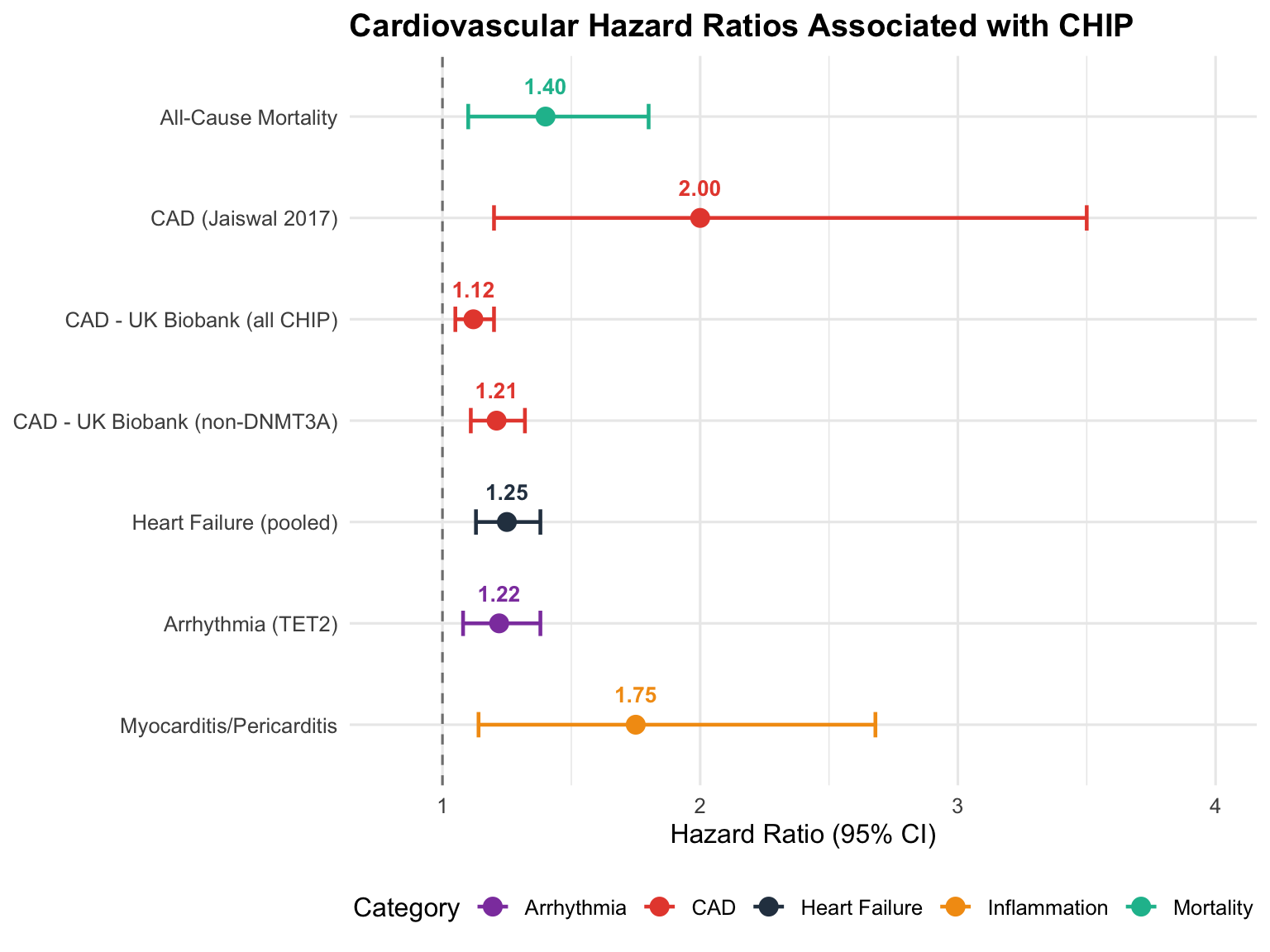
Two landmark 2014 studies demonstrated that CHIP was associated with a **1.4-fold increase in all-cause mortality** driven substantially by excess cardiovascular deaths [@Jaiswal2014; @Genovese2014]. A subsequent 2017 analysis confirmed an approximately **2-fold elevated hazard for incident coronary artery disease** [@Jaiswal2017]. Validation in the UK Biobank demonstrated a hazard ratio of 1.12 (95% CI 1.05–1.20) for a composite CAD endpoint, rising to 1.21 for non-DNMT3A mutations [@Vlasschaert2023ukbb; @Vlasschaert2023circ].
In vivo mouse experiments and longitudinal human cohort studies have established a **causal relationship** between CHIP and atherosclerotic cardiovascular disease, mediated by NLRP3 inflammasome-driven IL-1β and IL-6 secretion from mutant macrophages [@Fuster2017; @Bick2020circ]. Prospective longitudinal data suggests a **unidirectional relationship** where CHIP drives de novo atherosclerosis, while existing atherosclerosis does not significantly alter clonal trajectories [@Diez2024].
Heart failure represents a second major cardiovascular consequence, with a pooled hazard ratio of **1.25 (95% CI 1.13–1.38)** for incident heart failure among CHIP carriers [@Yu2021; @Schuermans2024hf]. CHIP is also associated with cardiac arrhythmias, myocarditis, and pericarditis.
```{r}
#| label: fig-cv-hazard-ratios
#| fig-cap: "Hazard ratios for cardiovascular outcomes associated with CHIP from major studies."
library(ggplot2)

cv_data <- data.frame(
  outcome = c("All-Cause Mortality", "CAD (Jaiswal 2017)",
              "CAD - UK Biobank (all CHIP)", "CAD - UK Biobank (non-DNMT3A)",
              "Heart Failure (pooled)", "Arrhythmia (TET2)",
              "Myocarditis/Pericarditis"),
  hr = c(1.4, 2.0, 1.12, 1.21, 1.25, 1.22, 1.75),
  hr_lo = c(1.1, 1.2, 1.05, 1.11, 1.13, 1.08, 1.14),
  hr_hi = c(1.8, 3.5, 1.20, 1.32, 1.38, 1.38, 2.68),
  category = c("Mortality", "CAD", "CAD", "CAD", "Heart Failure", "Arrhythmia", "Inflammation")
)

cv_data$outcome <- factor(cv_data$outcome, levels = rev(cv_data$outcome))

ggplot(cv_data, aes(x = hr, y = outcome, color = category)) +
  geom_vline(xintercept = 1, linetype = "dashed", color = "grey50") +
  geom_point(size = 3.5) +
  geom_errorbarh(aes(xmin = hr_lo, xmax = hr_hi), height = 0.25, linewidth = 0.8) +
  geom_text(aes(label = sprintf("%.2f", hr)), nudge_y = 0.3, size = 3.5, fontface = "bold") +
  scale_color_manual(values = c("#8E44AD", "#E74C3C", "#2C3E50", "#F39C12", "#1ABC9C")) +
  labs(
    x = "Hazard Ratio (95% CI)",
    y = NULL,
    title = "Cardiovascular Hazard Ratios Associated with CHIP",
    color = "Category"
  ) +
  theme_minimal(base_size = 12) +
  theme(
    plot.title = element_text(face = "bold"),
    legend.position = "bottom"
  ) +
  xlim(0.8, 4.0)
```
### Other Clinical Consequences
CHIP's clinical significance extends well beyond the cardiovascular system. Associations include ischemic stroke, severe COVID-19, progressive chronic kidney disease, chronic liver disease, and inflammatory conditions including rheumatoid arthritis and ulcerative colitis.
A particularly important emerging area is the role of CH in solid-organ malignancy. CHIP is present in the blood of approximately **1 in 4 solid tumor patients** — higher than age-matched controls. Tumor-infiltrating CHIP (where mutant immune cells migrate into the tumor microenvironment) has been independently shown by multiple groups to confer shorter progression-free survival and decreased overall survival [@Pich2025].
### Inflammation as the Unifying Mechanism
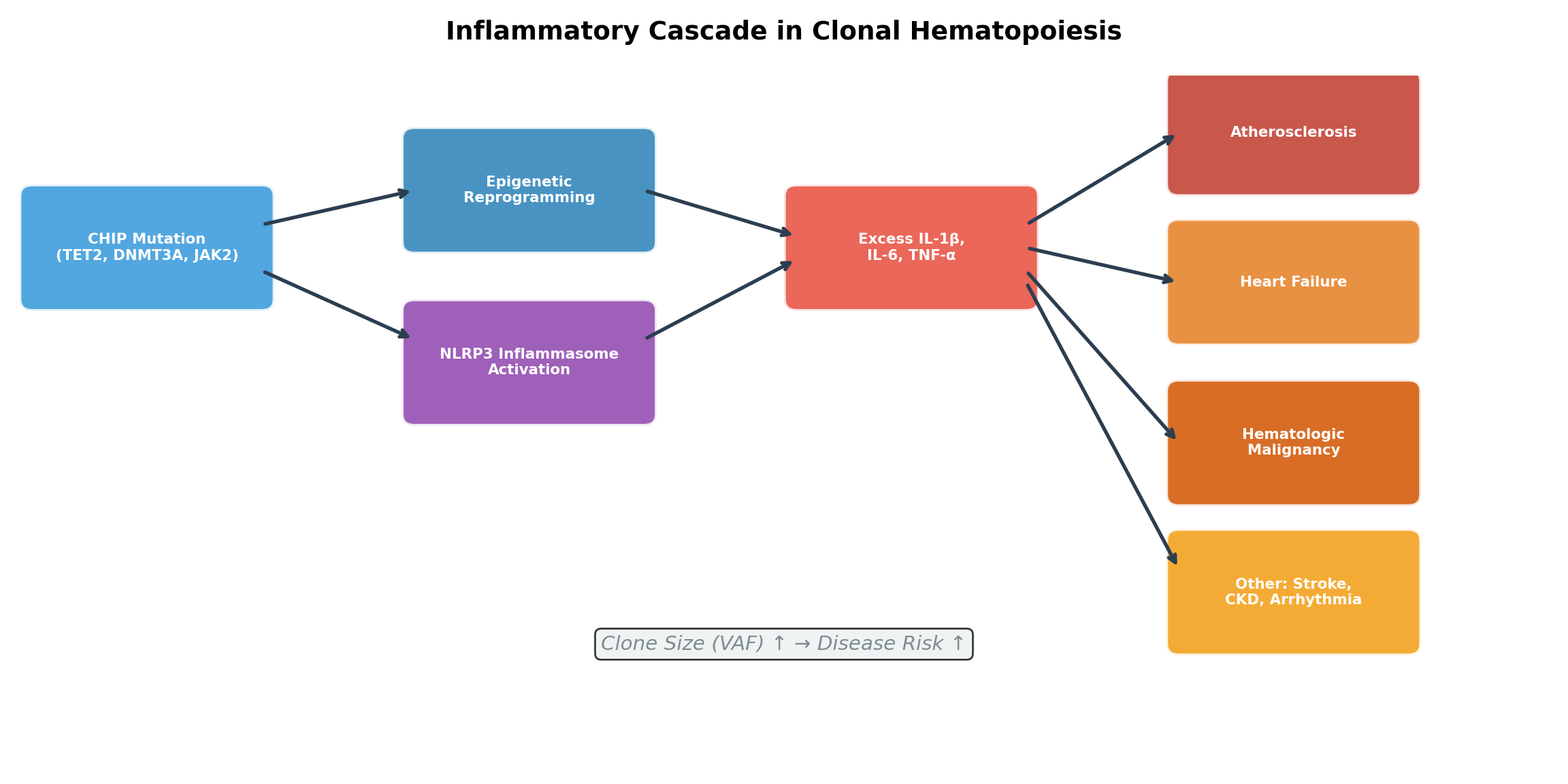
Inflammation is the mechanistic thread unifying the diverse clinical associations of CHIP [@Cai2018; @Fuster2017]:
- **TET2/DNMT3A loss-of-function**: Reprogram immune cell epigenetics → enhanced proinflammatory cytokine transcription → NLRP3 inflammasome sensitization
- **JAK2 V617F**: Constitutive JAK-STAT signaling → proinflammatory/prothrombotic monocytes → platelet-leukocyte aggregates
- **Dose-response**: Systemic inflammatory burden scales with clone size (VAF), creating a dose-response relationship with disease risk [@Ezzat2025]
```{python}
#| label: fig-inflammation-pathway
#| fig-cap: "Schematic of the inflammatory cascade driven by CHIP mutations in TET2, DNMT3A, and JAK2."
import matplotlib.pyplot as plt
import matplotlib.patches as mpatches

fig, ax = plt.subplots(figsize=(12, 6))
ax.set_xlim(0, 12)
ax.set_ylim(0, 6)
ax.axis('off')
# Boxes
boxes = {
    'CHIP Mutation\n(TET2, DNMT3A, JAK2)': (1, 4.5, '#3498DB'),
    'Epigenetic\nReprogramming': (4, 5, '#2980B9'),
    'NLRP3 Inflammasome\nActivation': (4, 3.5, '#8E44AD'),
    'Excess IL-1β,\nIL-6, TNF-α': (7, 4.5, '#E74C3C'),
    'Atherosclerosis': (10, 5.5, '#C0392B'),
    'Heart Failure': (10, 4.2, '#E67E22'),
    'Hematologic\nMalignancy': (10, 2.8, '#D35400'),
    'Other: Stroke,\nCKD, Arrhythmia': (10, 1.5, '#F39C12'),
}

for label, (x, y, color) in boxes.items():
    rect = mpatches.FancyBboxPatch((x-0.9, y-0.45), 1.8, 0.9,
                                     boxstyle="round,pad=0.1",
                                     facecolor=color, edgecolor='white',
                                     linewidth=2, alpha=0.85)
    ax.add_patch(rect)
    ax.text(x, y, label, ha='center', va='center', fontsize=8,
            color='white', fontweight='bold')

# Arrows
arrow_props = dict(arrowstyle='->', color='#2C3E50', lw=2)
ax.annotate('', xy=(3.1, 5), xytext=(1.9, 4.7), arrowprops=arrow_props)
ax.annotate('', xy=(3.1, 3.7), xytext=(1.9, 4.3), arrowprops=arrow_props)
ax.annotate('', xy=(6.1, 4.6), xytext=(4.9, 5), arrowprops=arrow_props)
ax.annotate('', xy=(6.1, 4.4), xytext=(4.9, 3.7), arrowprops=arrow_props)
ax.annotate('', xy=(9.1, 5.5), xytext=(7.9, 4.7), arrowprops=arrow_props)
ax.annotate('', xy=(9.1, 4.2), xytext=(7.9, 4.5), arrowprops=arrow_props)
ax.annotate('', xy=(9.1, 2.8), xytext=(7.9, 4.3), arrowprops=arrow_props)
ax.annotate('', xy=(9.1, 1.7), xytext=(7.9, 4.2), arrowprops=arrow_props)

# Clone size annotation
ax.annotate('Clone Size (VAF) ↑ → Disease Risk ↑',
            xy=(6, 1), fontsize=11, fontstyle='italic', color='#7F8C8D',
            ha='center',
            bbox=dict(boxstyle='round', facecolor='#ECF0F1', alpha=0.8))

ax.set_title('Inflammatory Cascade in Clonal Hematopoiesis', fontsize=14, fontweight='bold', pad=20)

plt.tight_layout()
plt.savefig("inflammation.png", dpi=150, bbox_inches='tight')
plt.show()
```
## Current Management and Therapies {#sec-management}
Despite growing recognition, management of CH remains largely observational with no FDA-approved therapies. Current NCCN guidelines recommend [@Greenberg2025]:
| CH Status | Surveillance | Frequency |
|:----------------------|:--------------------------|:----------------------|
| CHIP without cytopenia | Observation + CBC | Every 3–6 months |
| Lower-risk CCUS | Annual monitoring | Annually |
| High-risk CCUS | Intensive surveillance + clinical trial consideration | CBC 2–4×/year |
Dedicated CH clinics provide multidisciplinary care incorporating hematology, cardiology, and cardio-oncology. For CH-associated cardiovascular risk, management focuses on aggressive modification of traditional risk factors (hypertension, hyperlipidemia, diabetes, obesity, tobacco) and inflammatory biomarker measurement (hs-CRP, IL-6).
## Investigational Therapies {#sec-therapies}
Developing CH therapies is challenged by the low absolute progression risk (0.5–1%/year). Surrogate endpoints under consideration include VAF changes, cytopenias, inflammatory biomarkers, and cardiovascular imaging endpoints [@Haque2025].
### Anti-Inflammatory Therapies
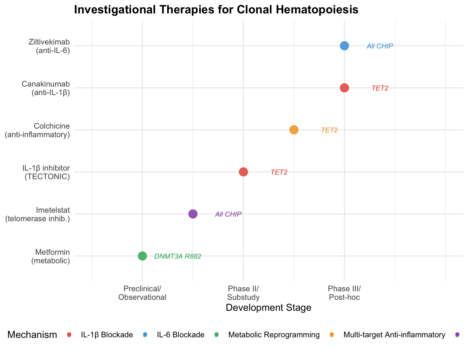
The most advanced strategy leverages the central role of inflammasome-driven inflammation:
- **Canakinumab** (IL-1β blockade): CANTOS trial post-hoc analysis showed TET2 CHIP carriers derived the greatest cardiovascular benefit [@Svensson2022]
- **Colchicine**: LoDoCo2 substudy showed attenuated clonal expansion in TET2 CH — 14.9% annual increase on placebo vs. 6.3% with colchicine [@Mohammadnia2025]
- **Ziltivekimab** (anti-IL-6): HERMES trial (NCT05636176) ongoing
- **TECTONIC trial** (NCT06691217): Prospectively testing IL-1β inhibition in TET2 CHIP
### Repurposed Agents
- **Metformin**: Experimental evidence for reducing *DNMT3A* R882 clonal expansion, though observational data from the Women's Health Initiative did not confirm clinical effect
- **Statins**: May modulate inflammatory signaling
```{r}
#| label: fig-trial-landscape
#| fig-cap: "Landscape of investigational therapies for clonal hematopoiesis, organized by therapeutic mechanism."
library(ggplot2)

trials <- data.frame(
  therapy = c("Canakinumab\n(anti-IL-1β)", "Colchicine\n(anti-inflammatory)",
              "Ziltivekimab\n(anti-IL-6)", "IL-1β inhibitor\n(TECTONIC)",
              "Metformin\n(metabolic)", "Imetelstat\n(telomerase inhib.)"),
  mechanism = c("IL-1β Blockade", "Multi-target Anti-inflammatory",
                "IL-6 Blockade", "IL-1β Blockade",
                "Metabolic Reprogramming", "Telomere Biology"),
  stage = c(3, 2.5, 3, 2, 1, 1.5),
  evidence = c("Post-hoc CANTOS", "LoDoCo2 Substudy",
               "HERMES (ongoing)", "NCT06691217 (ongoing)",
               "Preclinical + Observational", "Preclinical"),
  target_gene = c("TET2", "TET2", "All CHIP", "TET2", "DNMT3A R882", "All CHIP")
)

ggplot(trials, aes(x = stage, y = reorder(therapy, stage),
                   color = mechanism, size = 4)) +
  geom_point(alpha = 0.8) +
  geom_text(aes(label = target_gene), nudge_x = 0.35, size = 3, fontface = "italic") +
  scale_x_continuous(
    breaks = 1:3,
    labels = c("Preclinical/\nObservational", "Phase II/\nSubstudy", "Phase III/\nPost-hoc"),
    limits = c(0.5, 4)
  ) +
  scale_color_manual(values = c("#E74C3C", "#3498DB", "#27AE60", "#F39C12", "#8E44AD", "#2C3E50")) +
  labs(
    x = "Development Stage",
    y = NULL,
    title = "Investigational Therapies for Clonal Hematopoiesis",
    color = "Mechanism"
  ) +
  guides(size = "none") +
  theme_minimal(base_size = 12) +
  theme(
    plot.title = element_text(face = "bold"),
    legend.position = "bottom"
  )
```
# Methods for Discovery of Therapeutics {#sec-methods}
The development of effective CH therapeutic strategies requires a principled framework organized along three converging lines: (1) genetic and environmental determinants of CH acquisition, (2) factors modulating clonal expansion and disease progression, and (3) computational tools for unbiased therapeutic target discovery.
## Risk and Resilience Mechanisms to CH Acquisition {#sec-gwas}
Genome-wide association studies (GWAS) identify the inherited genetic architecture of CH susceptibility. Human genetic evidence significantly increases the probability of clinical success in drug development [@Nelson2015; @Minikel2024].
Key GWAS findings include:
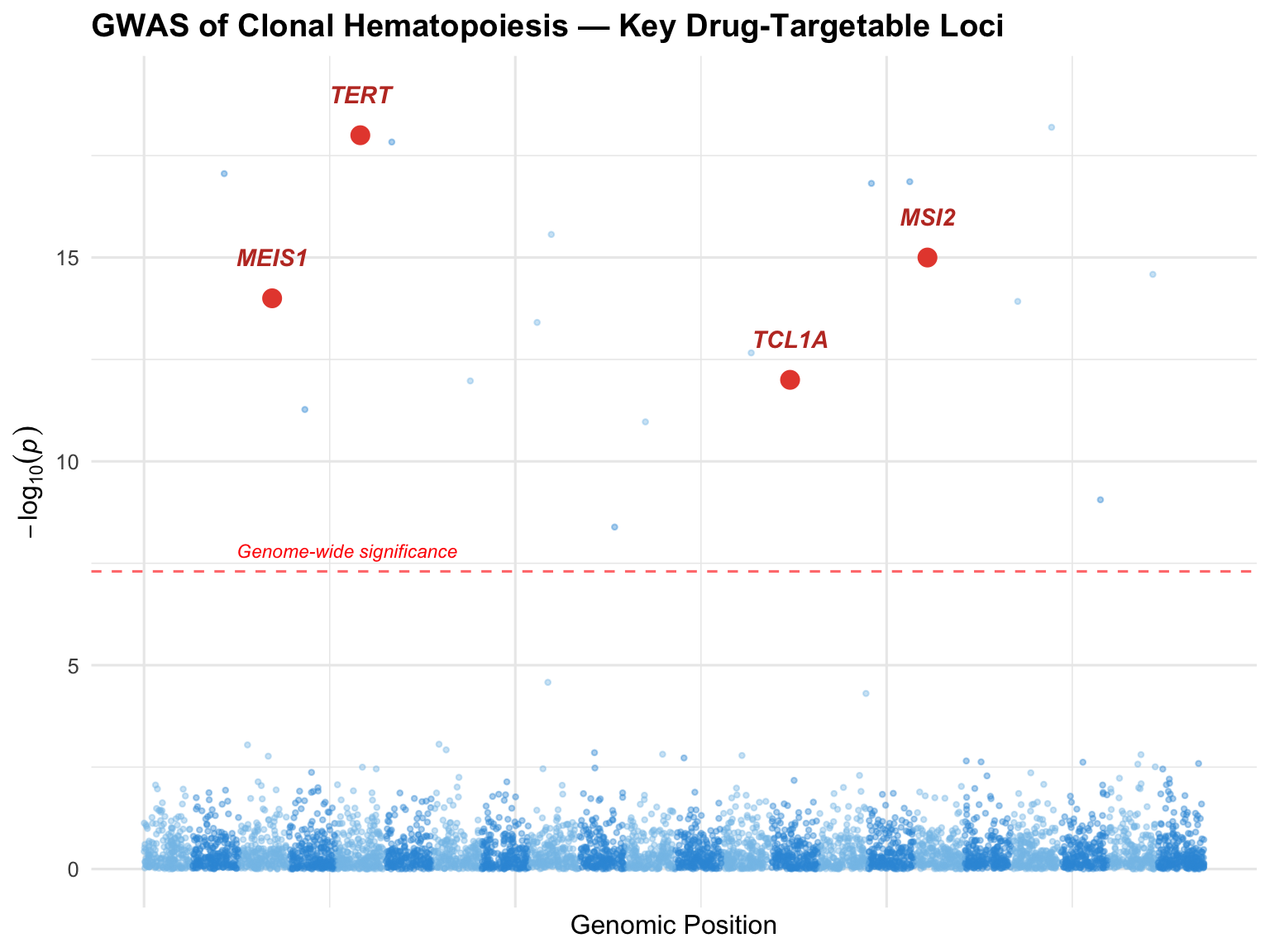
- **rs7705526 (TERT promoter)**: Predisposes to clonal expansion across multiple CH driver genes via telomere length maintenance. Mendelian randomization confirmed that shorter germline telomere length increases CH susceptibility.
- **rs17834140 (MSI2)**: Protective variant that down-regulates Musashi-2 in HSPCs by disrupting a GATA2 binding site, reducing CHIP-mutant HSPC proliferation. Nominates MSI2 as a therapeutic target [@Agarwal2026; @Kessler2022].
- Over **60 significant loci** have been identified for CH overall (both CHIP and mCAs) across large-scale GWAS meta-analyses [@Bick2020nat].
Environmental factors modulating acquisition include tobacco smoking, cytotoxic chemotherapy, ionizing radiation, and occupational particulate exposure [@Bolton2020].
```{r}
#| label: fig-gwas-manhattan
#| fig-cap: "Simulated Manhattan-style plot illustrating key GWAS loci for clonal hematopoiesis susceptibility. Highlighted loci represent validated drug-targetable genes."
library(ggplot2)

set.seed(42)
n_snps <- 5000
chr <- sample(1:22, n_snps, replace = TRUE,
              prob = c(rep(1, 22)))
pos <- runif(n_snps, 0, 250e6)
pval <- runif(n_snps, 0, 1)

# Make most SNPs non-significant
logp <- -log10(pval)

# Add some significant hits
sig_idx <- sample(1:n_snps, 15)
logp[sig_idx] <- runif(15, 8, 20)

# Add key labeled loci
key_loci <- data.frame(
  chr = c(5, 17, 14, 3),
  pos = c(125e6, 60e6, 100e6, 170e6),
  logp = c(18, 15, 12, 14),
  gene = c("TERT", "MSI2", "TCL1A", "MEIS1")
)

gwas_df <- data.frame(chr = chr, pos = pos, logp = logp)
gwas_df$x_pos <- gwas_df$pos + (gwas_df$chr - 1) * 260e6

key_loci$x_pos <- key_loci$pos + (key_loci$chr - 1) * 260e6

ggplot() +
  geom_point(data = gwas_df,
             aes(x = x_pos / 1e9, y = logp, color = factor(chr %% 2)),
             alpha = 0.4, size = 0.8) +
  geom_point(data = key_loci, aes(x = x_pos / 1e9, y = logp),
             color = "#E74C3C", size = 3.5) +
  geom_text(data = key_loci, aes(x = x_pos / 1e9, y = logp + 1, label = gene),
            fontface = "bold.italic", size = 3.8, color = "#C0392B") +
  geom_hline(yintercept = -log10(5e-8), linetype = "dashed", color = "red", alpha = 0.6) +
  scale_color_manual(values = c("#3498DB", "#85C1E9")) +
  labs(
    x = "Genomic Position",
    y = expression(-log[10](italic(p))),
    title = "GWAS of Clonal Hematopoiesis — Key Drug-Targetable Loci"
  ) +
  theme_minimal(base_size = 12) +
  theme(
    legend.position = "none",
    plot.title = element_text(face = "bold"),
    axis.text.x = element_blank()
  ) +
  annotate("text", x = 0.5, y = -log10(5e-8) + 0.5,
           label = "Genome-wide significance", color = "red",
           size = 3, hjust = 0, fontface = "italic")
```
## Risk and Resilience Mechanisms to Clonal Expansion {#sec-expansion}
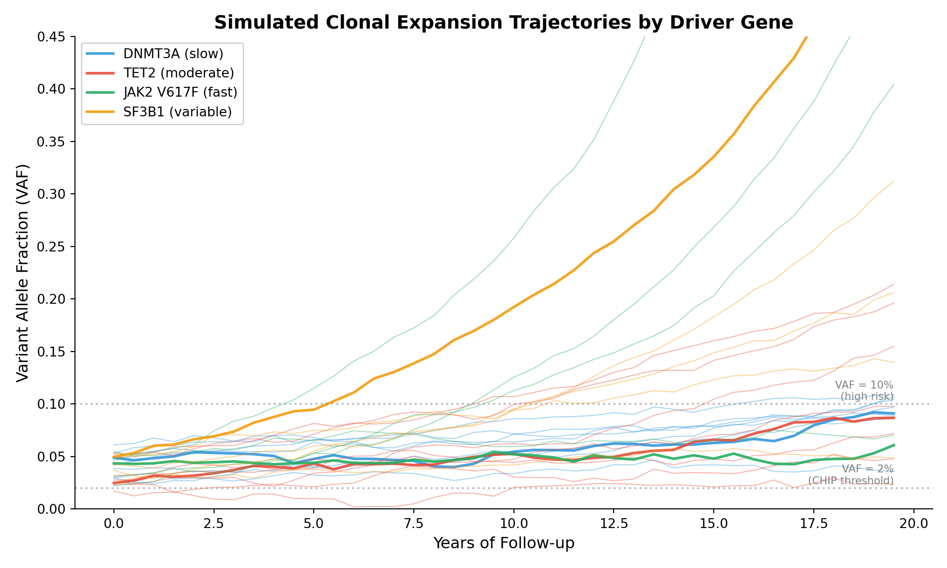
Once a driver mutation is established, the expansion rate — reflecting the fitness advantage of a mutation in a specific host environment — is a critical clinical variable. Three primary approaches measure expansion:
1. **Single-timepoint inference**: Using VAF as a proxy for expansion history
2. **PACER (Passenger-Approximated Clonal Expansion Rate)**: Leverages "clock-like" passenger mutations to infer a clonal "birth date" from a single blood draw [@Watson2020; @Pershad2024mca]
3. **Longitudinal sequencing**: Serial VAF/CF measurements over time (gold standard)
```{r}
#| label: tbl-longitudinal
#| tbl-cap: "Summary of major longitudinal CHIP sequencing studies."
library(knitr)

longitudinal_studies <- data.frame(
  Study = c("Fabre 2022", "Robertson 2022", "van Zeventer 2023",
            "Uddin 2024", "Mack & Pershad 2025", "Pershad 2025 (Ch. 3)"),
  Cohort = c("SardiNIA", "Lothian Birth Cohort", "Lifelines",
             "ARIC", "Vanderbilt BioVU", "Women's Health Initiative"),
  `CHIP / Total` = c("300 / 400", "70 / 1,500", "1,300 / 3,400",
                     "735 / 4,200", "711 / 3,000", "4,331 / 6,976"),
  `Follow-up` = c("13 yrs", "6 yrs", "3-4 yrs", "21 yrs", "6 yrs", "16 yrs"),
  Method = c("Targeted NGS", "Targeted NGS", "Targeted NGS",
             "WES", "Targeted NGS", "Targeted NGS")
)

kable(longitudinal_studies, align = "llccc")
```
A key GWAS result is the **rs2887399 variant in the TCL1A promoter**, which modifies expansion rate of TET2-mutant clones. In the wildtype setting with TET2 CHIP, the TCL1A promoter becomes aberrantly accessible, increasing TCL1A expression and clonal expansion. The rs2887399-T variant prevents this, attenuating expansion. This nominates **TCL1A as a druggable target** for TET2 CHIP.
```{python}
#| label: fig-clonal-trajectories
#| fig-cap: "Simulated clonal expansion trajectories showing heterogeneity in growth rates across different CHIP driver genes."
import numpy as np
import matplotlib.pyplot as plt

np.random.seed(42)
years = np.arange(0, 20, 0.5)

fig, ax = plt.subplots(figsize=(10, 6))

# Different driver genes with characteristic growth rates
drivers = {
    'DNMT3A (slow)': {'mean_rate': 0.03, 'n': 8, 'color': '#3498DB'},
    'TET2 (moderate)': {'mean_rate': 0.06, 'n': 8, 'color': '#E74C3C'},
    'JAK2 V617F (fast)': {'mean_rate': 0.10, 'n': 5, 'color': '#27AE60'},
    'SF3B1 (variable)': {'mean_rate': 0.07, 'n': 5, 'color': '#F39C12'},
}

for driver, params in drivers.items():
    for i in range(params['n']):
        rate = np.random.normal(params['mean_rate'], params['mean_rate'] * 0.5)
        init_vaf = np.random.uniform(0.02, 0.06)
        noise = np.cumsum(np.random.normal(0, 0.003, len(years)))
        trajectory = init_vaf * np.exp(rate * years) + noise
        trajectory = np.clip(trajectory, 0.001, 0.5)

        alpha = 0.4 if i > 0 else 0.9
        lw = 0.8 if i > 0 else 2.0
        label = driver if i == 0 else None
        ax.plot(years, trajectory, color=params['color'], alpha=alpha,
                linewidth=lw, label=label)

ax.axhline(y=0.02, linestyle=':', color='grey', alpha=0.5)
ax.text(19.5, 0.022, 'VAF = 2%\n(CHIP threshold)', fontsize=8,
        color='grey', ha='right', va='bottom')
ax.axhline(y=0.10, linestyle=':', color='grey', alpha=0.5)
ax.text(19.5, 0.102, 'VAF = 10%\n(high risk)', fontsize=8,
        color='grey', ha='right', va='bottom')

ax.set_xlabel('Years of Follow-up', fontsize=12)
ax.set_ylabel('Variant Allele Fraction (VAF)', fontsize=12)
ax.set_title('Simulated Clonal Expansion Trajectories by Driver Gene',
             fontsize=14, fontweight='bold')
ax.legend(loc='upper left', fontsize=10, framealpha=0.9)
ax.set_ylim(0, 0.45)
ax.spines['top'].set_visible(False)
ax.spines['right'].set_visible(False)

plt.tight_layout()
plt.savefig("trajectories.png", dpi=150, bbox_inches='tight')
plt.show()
```
## In Silico Perturbation as an Emerging Therapeutic Discovery Method {#sec-insilico}
A fundamental limitation of epidemiological and candidate-gene approaches is their dependence on existing human genetic variation, drug exposures, and prior biological knowledge. This mechanism-first paradigm is inherently biased toward targets with existing mechanistic understanding — which, for most of the 75 CHIP driver genes, remains incomplete.
### Single-Cell Foundation Models (scFMs)
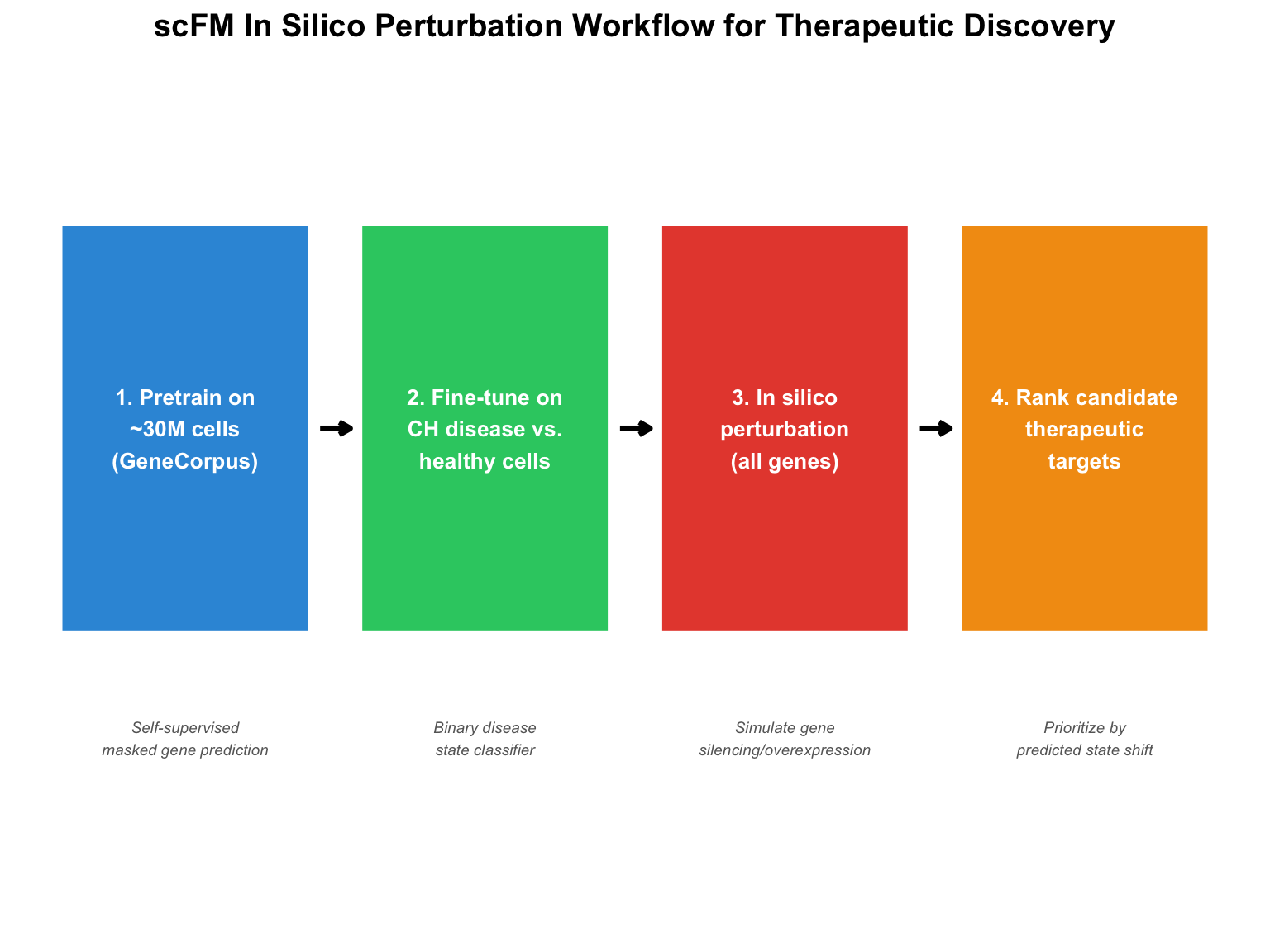
Analogous to large language models (LLMs) in NLP, scFMs are deep neural networks pretrained on tens to hundreds of millions of single-cell transcriptomic profiles using self-supervised objectives [@Theodoris2023; @Cui2024]. The paradigmatic scFM, **Geneformer**, was pretrained on the GeneCorpus (\~30 million single-cell profiles) using a masked gene prediction objective.
### In Silico Perturbation
In silico perturbation uses scFMs to computationally simulate the transcriptional consequences of silencing or overexpressing individual genes — analogous to a genome-wide CRISPR screen (Perturb-Seq) [@Dixit2016; @Pershad2025geneformer]. By fine-tuning on disease-relevant transcriptomic profiles, one can rank candidate therapeutic targets by predicted magnitude of state shift toward a healthy phenotype.
However, critics have found that simpler traditional models (e.g., linear regression) that do not require pretraining may perform comparably. Chapter 6 of the dissertation benchmarks Geneformer's in silico perturbation using genome-wide CRISPR screens and develops methods to improve prediction accuracy via learning from Perturb-Seq examples.
```{r}
#| label: fig-scfm-workflow
#| fig-cap: "Workflow for in silico perturbation using single-cell foundation models. The model is pretrained on large-scale scRNA-seq data, fine-tuned on disease-specific data, then used to computationally simulate gene perturbations."
library(ggplot2)
library(grid)

steps <- data.frame(
  step = c("1. Pretrain on\n~30M cells\n(GeneCorpus)",
           "2. Fine-tune on\nCH disease vs.\nhealthy cells",
           "3. In silico\nperturbation\n(all genes)",
           "4. Rank candidate\ntherapeutic\ntargets"),
  x = 1:4,
  y = rep(1, 4),
  color = c("#3498DB", "#2ECC71", "#E74C3C", "#F39C12")
)

ggplot(steps, aes(x = x, y = y)) +
  geom_tile(aes(fill = color), width = 0.85, height = 0.6,
            color = "white", linewidth = 2) +
  geom_text(aes(label = step), size = 3.5, fontface = "bold", color = "white") +
  scale_fill_identity() +
  # Arrows between steps
  annotate("segment", x = 1.45, xend = 1.55, y = 1, yend = 1,
           arrow = arrow(length = unit(0.2, "cm")), linewidth = 1.2) +
  annotate("segment", x = 2.45, xend = 2.55, y = 1, yend = 1,
           arrow = arrow(length = unit(0.2, "cm")), linewidth = 1.2) +
  annotate("segment", x = 3.45, xend = 3.55, y = 1, yend = 1,
           arrow = arrow(length = unit(0.2, "cm")), linewidth = 1.2) +
  # Method labels below
  annotate("text", x = 1, y = 0.55, label = "Self-supervised\nmasked gene prediction",
           size = 2.5, color = "grey40", fontface = "italic") +
  annotate("text", x = 2, y = 0.55, label = "Binary disease\nstate classifier",
           size = 2.5, color = "grey40", fontface = "italic") +
  annotate("text", x = 3, y = 0.55, label = "Simulate gene\nsilencing/overexpression",
           size = 2.5, color = "grey40", fontface = "italic") +
  annotate("text", x = 4, y = 0.55, label = "Prioritize by\npredicted state shift",
           size = 2.5, color = "grey40", fontface = "italic") +
  labs(title = "scFM In Silico Perturbation Workflow for Therapeutic Discovery") +
  theme_void(base_size = 12) +
  theme(plot.title = element_text(face = "bold", hjust = 0.5)) +
  coord_cartesian(ylim = c(0.3, 1.5))
```
# Computational Tools & Worked Examples {#sec-tools}
## VAF Detection Power Calculations in R
A key concept from the dissertation is understanding how sequencing depth affects the ability to detect somatic variants at a given VAF. Here we compute the probability of observing ≥ *k* mutant reads at a given depth and VAF:
```{r}
#| label: fig-power-calc
#| fig-cap: "Statistical power to detect a somatic variant (requiring ≥3 mutant reads) as a function of sequencing depth and VAF."
library(ggplot2)

# Power calculation: P(X >= k) where X ~ Binom(depth, VAF)
calc_power <- function(depth, vaf, min_reads = 3) {
  1 - pbinom(min_reads - 1, size = depth, prob = vaf)
}

depths <- c(30, 100, 500, 2000, 5000)
vafs <- seq(0.001, 0.10, by = 0.001)

power_df <- expand.grid(depth = depths, vaf = vafs)
power_df$power <- mapply(calc_power, power_df$depth, power_df$vaf)
power_df$depth_label <- paste0(power_df$depth, "×")
power_df$depth_label <- factor(power_df$depth_label,
                                levels = paste0(depths, "×"))

ggplot(power_df, aes(x = vaf * 100, y = power * 100,
                     color = depth_label, group = depth_label)) +
  geom_line(linewidth = 1.2) +
  geom_hline(yintercept = 80, linetype = "dashed", color = "grey50", alpha = 0.7) +
  annotate("text", x = 8, y = 82, label = "80% power threshold",
           color = "grey50", size = 3, fontface = "italic") +
  scale_color_viridis_d(option = "plasma", end = 0.9) +
  labs(
    x = "Variant Allele Fraction (%)",
    y = "Detection Power (%)",
    title = "Sequencing Depth vs. Detection Power",
    subtitle = "Requiring ≥ 3 mutant reads (binomial model)",
    color = "Depth"
  ) +
  theme_minimal(base_size = 13) +
  theme(
    plot.title = element_text(face = "bold"),
    legend.position = "right"
  )
```
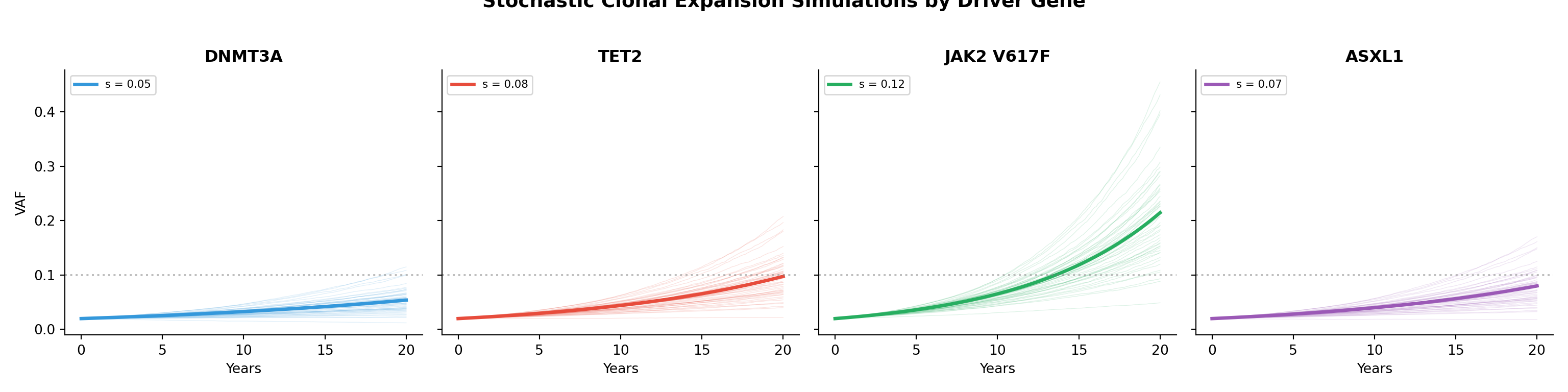
## Simulating Clonal Dynamics in Python
Using a simple exponential growth model with stochastic noise to simulate how clones expand over time:
```{python}
#| label: fig-clone-sim
#| fig-cap: "Stochastic simulation of clonal dynamics. Each panel shows 50 independent simulations for a given driver gene's characteristic fitness advantage."
import numpy as np
import matplotlib.pyplot as plt

def simulate_clone(s, t_max=20, dt=0.1, vaf_init=0.02, sigma=0.01):
    """Simulate clonal expansion using a Wright-Fisher-inspired model.

    Parameters:
        s: selection coefficient (fitness advantage)
        t_max: max time in years
        dt: time step
        vaf_init: initial VAF
        sigma: noise scale
    """
    steps = int(t_max / dt)
    vaf = np.zeros(steps)
    vaf[0] = vaf_init
    for i in range(1, steps):
        drift = np.random.normal(0, sigma * np.sqrt(dt))
        vaf[i] = vaf[i-1] * (1 + s * dt) + drift * vaf[i-1]
        vaf[i] = np.clip(vaf[i], 0.001, 0.50)
    return np.linspace(0, t_max, steps), vaf

genes = {
    'DNMT3A': {'s': 0.05, 'color': '#3498DB'},
    'TET2': {'s': 0.08, 'color': '#E74C3C'},
    'JAK2 V617F': {'s': 0.12, 'color': '#27AE60'},
    'ASXL1': {'s': 0.07, 'color': '#9B59B6'}
}

fig, axes = plt.subplots(1, 4, figsize=(16, 4), sharey=True)

for ax, (gene, params) in zip(axes, genes.items()):
    np.random.seed(42)
    for i in range(50):
        t, v = simulate_clone(params['s'] + np.random.normal(0, 0.02))
        ax.plot(t, v, color=params['color'], alpha=0.15, linewidth=0.5)

    # Median trajectory
    t, v_med = simulate_clone(params['s'], sigma=0)
    ax.plot(t, v_med, color=params['color'], linewidth=2.5, label=f's = {params["s"]}')

    ax.axhline(y=0.10, linestyle=':', color='grey', alpha=0.5)
    ax.set_title(gene, fontsize=12, fontweight='bold')
    ax.set_xlabel('Years')
    ax.legend(fontsize=8, loc='upper left')
    ax.spines['top'].set_visible(False)
    ax.spines['right'].set_visible(False)

axes[0].set_ylabel('VAF')
fig.suptitle('Stochastic Clonal Expansion Simulations by Driver Gene',
             fontsize=14, fontweight='bold', y=1.02)
plt.tight_layout()
plt.savefig("clone_sim.png", dpi=150, bbox_inches='tight')
plt.show()
```
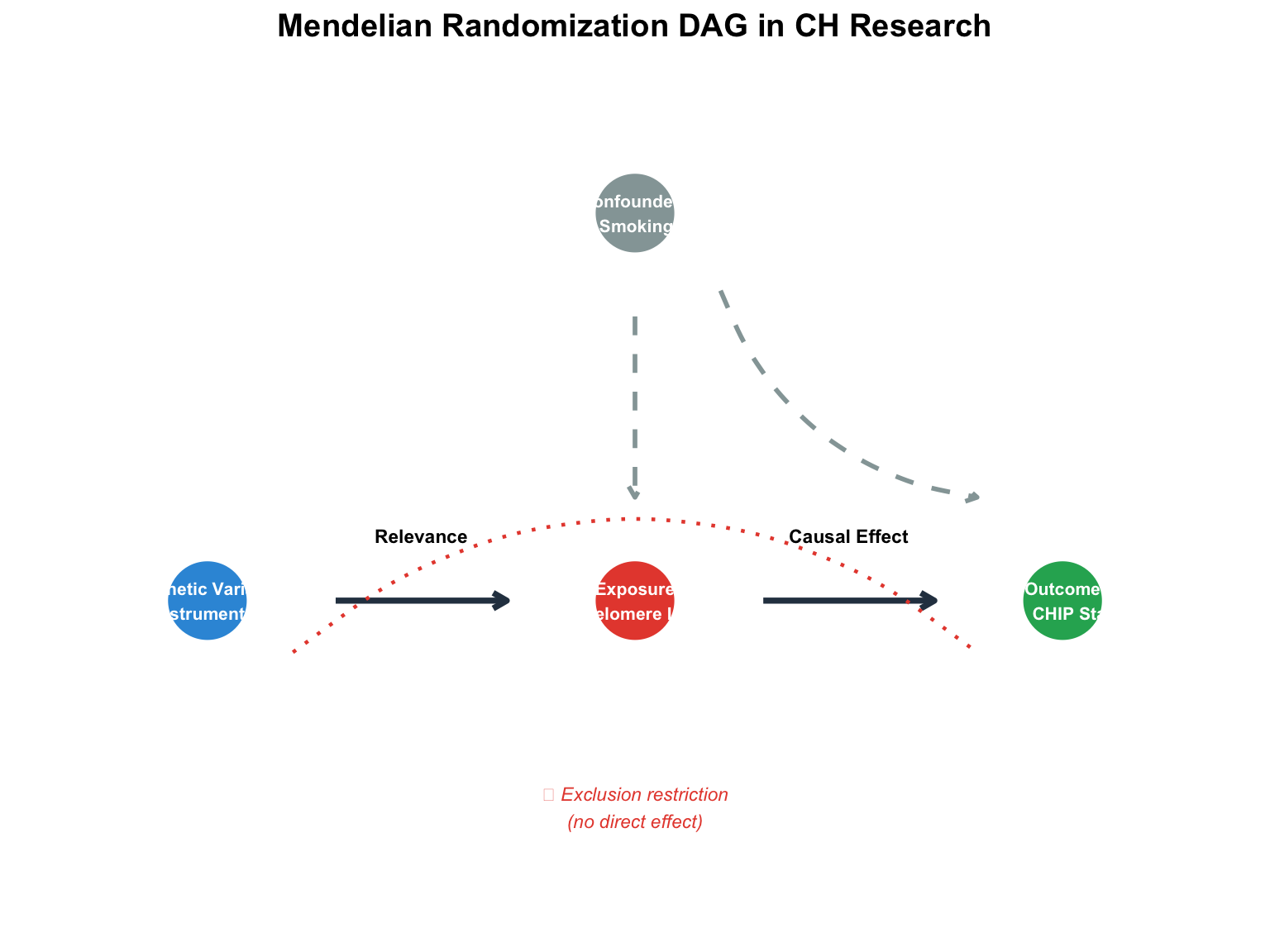
## Mendelian Randomization Conceptual Framework in R
Mendelian randomization (MR) has been instrumental in establishing causal relationships in CH biology, such as confirming shorter telomere length increases CH susceptibility and that IL-6 signaling mediates cardiovascular risk [@Bick2020circ; @Vlasschaert2023circ]:
```{r}
#| label: fig-mr-dag
#| fig-cap: "Directed acyclic graph (DAG) illustrating the Mendelian randomization framework used to assess causal effects in clonal hematopoiesis research. Genetic instruments (Z) must satisfy the three core IV assumptions."
library(ggplot2)

dag_nodes <- data.frame(
  label = c("Genetic Variant\n(Instrument Z)", "Exposure\n(e.g., Telomere Length)",
            "Outcome\n(e.g., CHIP Status)", "Confounders\n(Age, Smoking, etc.)"),
  x = c(1, 3, 5, 3),
  y = c(2, 2, 2, 3.5),
  color = c("#3498DB", "#E74C3C", "#27AE60", "#95A5A6")
)

ggplot(dag_nodes, aes(x = x, y = y)) +
  # Causal path
  annotate("segment", x = 1.6, xend = 2.4, y = 2, yend = 2,
           arrow = arrow(length = unit(0.25, "cm")), linewidth = 1.3, color = "#2C3E50") +
  annotate("segment", x = 3.6, xend = 4.4, y = 2, yend = 2,
           arrow = arrow(length = unit(0.25, "cm")), linewidth = 1.3, color = "#2C3E50") +
  # Confounder paths (dashed)
  annotate("segment", x = 3, xend = 3, y = 3.1, yend = 2.4,
           arrow = arrow(length = unit(0.2, "cm")), linewidth = 1,
           color = "#95A5A6", linetype = "dashed") +
  annotate("curve", x = 3.4, xend = 4.6, y = 3.2, yend = 2.4,
           arrow = arrow(length = unit(0.2, "cm")), linewidth = 1,
           color = "#95A5A6", linetype = "dashed", curvature = 0.3) +
  # No direct path from Z to Y (crossed out)
  annotate("curve", x = 1.4, xend = 4.6, y = 1.8, yend = 1.8,
           linewidth = 0.8, color = "#E74C3C", linetype = "dotted", curvature = -0.4) +
  annotate("text", x = 3, y = 1.2, label = "✗ Exclusion restriction\n(no direct effect)",
           color = "#E74C3C", size = 3, fontface = "italic") +
  # Nodes
  geom_point(size = 16, aes(color = color)) +
  geom_text(aes(label = label), size = 2.8, fontface = "bold", color = "white") +
  scale_color_identity() +
  # Annotations
  annotate("text", x = 2, y = 2.25, label = "Relevance", size = 3, fontface = "bold") +
  annotate("text", x = 4, y = 2.25, label = "Causal Effect", size = 3, fontface = "bold") +
  labs(title = "Mendelian Randomization DAG in CH Research") +
  theme_void(base_size = 12) +
  theme(plot.title = element_text(face = "bold", hjust = 0.5)) +
  coord_cartesian(xlim = c(0.3, 5.7), ylim = c(0.8, 4))
```
# Key Dissertation Chapters Overview {#sec-chapters}
This dissertation is organized into chapters that systematically address the fitness, fate, and function of clonal hematopoiesis:
| Chapter | Topic | Key Contribution |
|:-----------------|:----------------|:-----------------------------------|
| 2 | Detection Sensitivity | Shallow WGS/WES profoundly underestimates CH disease associations |
| 3 | Longitudinal Dynamics | Largest longitudinal CHIP study (\~7,000 women in WHI) |
| 4 | mCA Genetics | Largest GWAS meta-analysis and PheWAS of autosomal mCAs (\>1M individuals) |
| 5 | Risk Prediction | Improved risk scores using mutation-specific heterogeneity and DNA methylation |
| 6 | In Silico Perturbation | Benchmarking and improving scFM predictions for therapeutic discovery |
# References {.unnumbered}
::: {#refs}
:::
# Session Info {.appendix}
```{r}
#| label: session-info
sessionInfo()
```
```{python}
#| label: python-session
import sys
print(f"Python version: {sys.version}")
import numpy; print(f"NumPy: {numpy.__version__}")
import matplotlib; print(f"Matplotlib: {matplotlib.__version__}")
```