6 SIR9900 in VEXAS Syndrome
SIVEX Study Design Report — A Randomized, Double-Blind, Placebo-Controlled Phase II Study
Executive Summary
This report provides a comprehensive analysis of the SIVEX study design, including statistical power considerations, pharmacological rationale, safety margins, and competitive positioning within the VEXAS treatment landscape. All figures are generated programmatically using R (ggplot2 ecosystem) and Python (matplotlib/seaborn) for full reproducibility.
7 VEXAS Syndrome: Disease Background
7.1 Pathogenesis & Epidemiology
VEXAS (Vacuoles, E1 enzyme, X-linked, Autoinflammatory, Somatic) syndrome is a recently identified adult-onset autoinflammatory disorder first described in 2020 by Beck et al. (NEJM). It is caused by somatic mutations in the UBA1 gene — encoding the E1 ubiquitin-activating enzyme — arising in hematopoietic stem cells. The canonical mutations reside at codon 41 (p.Met41Thr, p.Met41Val, p.Met41Leu) or neighboring splice sites (c.118-1, c.118-2).
Key epidemiological data:
| Parameter | Value | Source |
|---|---|---|
| Prevalence in men aged 50+ | ~1 in 4,269 | Beck et al. JAMA 2023 |
| Prevalence in women aged 50+ | ~1 in 26,238 | Beck et al. JAMA 2023 |
| Estimated US cases (age 50+) | ~15,000 (~13,200 men) | NYU Langone 2023 |
| 5-year survival rate | ~63% | Georgin-Lavialle et al. 2022 |
7.2 Clinical Manifestations
The disease bridges rheumatologic and hematologic domains, presenting with a broad spectrum of clinical sequelae including cutaneous disease (neutrophilic dermatoses, vasculitic lesions), constitutional symptoms (fever, fatigue, weight loss), musculoskeletal involvement (chondritis, arthritis), ocular inflammation (uveitis, scleritis), pulmonary disease (alveolitis), venous thromboembolism, and progressive bone marrow failure with MDS overlap.
7.3 Current Treatment Landscape
Show code
import matplotlib
matplotlib.use('Agg')
import matplotlib.pyplot as plt
import matplotlib.patches as mpatches
import numpy as np

# ── Palette ──
NAVY, GOLD, TEAL, CORAL, SLATE = '#1A2744', '#CFB991', '#2D8A8A', '#C75B4A', '#6B7280'
LIGHT_GOLD, WHITE, GREEN = '#F5EDD8', '#FFFFFF', '#2D8A5E'

plt.rcParams.update({
    'font.family': 'sans-serif',
    'font.size': 10,
    'axes.titlesize': 13,
    'axes.labelsize': 11,
    'figure.facecolor': WHITE,
    'axes.facecolor': WHITE,
    'axes.edgecolor': '#CCCCCC',
})

treatments = [
    'Glucocorticoids', 'JAK Inhibitors', 'Anti-IL6',
    'Anti-IL1', 'Anti-TNF', 'HMA\n(Azacitidine)',
    'SIR9900\n(RIPK1i)'
]
anti_inflam    = [4.5, 3.5, 3.0, 2.0, 1.5, 2.0, 4.5]
disease_mod    = [1.0, 2.0, 1.0, 1.0, 0.5, 3.5, 4.0]
tolerability   = [1.5, 2.5, 3.5, 3.0, 3.0, 2.0, 4.0]
mechanism_spec = [0.5, 2.5, 2.0, 2.0, 1.5, 2.5, 5.0]

fig, ax = plt.subplots(figsize=(10, 5.5))
x = np.arange(len(treatments))
w = 0.18

ax.bar(x - 1.5*w, anti_inflam,    w, color=NAVY,  alpha=0.85, label='Anti-inflammatory Efficacy')
ax.bar(x - 0.5*w, disease_mod,    w, color=TEAL,  alpha=0.85, label='Disease Modification Potential')
ax.bar(x + 0.5*w, tolerability,   w, color=GOLD,  alpha=0.85, label='Tolerability Profile')
ax.bar(x + 1.5*w, mechanism_spec, w, color=CORAL, alpha=0.85, label='Mechanism Specificity')

ax.axvspan(5.6, 6.4, color=LIGHT_GOLD, alpha=0.4, zorder=0)
ax.set_xticks(x)
ax.set_xticklabels(treatments, fontsize=9)
ax.set_ylabel('Comparative Score (0–5)', fontweight='bold')
ax.set_title('VEXAS Treatment Landscape: Multi-Dimensional Comparison',
             fontweight='bold', color=NAVY, fontsize=13)
ax.set_ylim(0, 5.8)
(0.0, 5.8)Show code
ax.legend(ncol=2, frameon=True, facecolor=WHITE, edgecolor='#CCCCCC',
          loc='upper center', fontsize=8.5, bbox_to_anchor=(0.5, 1.0))
ax.spines['top'].set_visible(False)
ax.spines['right'].set_visible(False)
plt.tight_layout()
plt.show()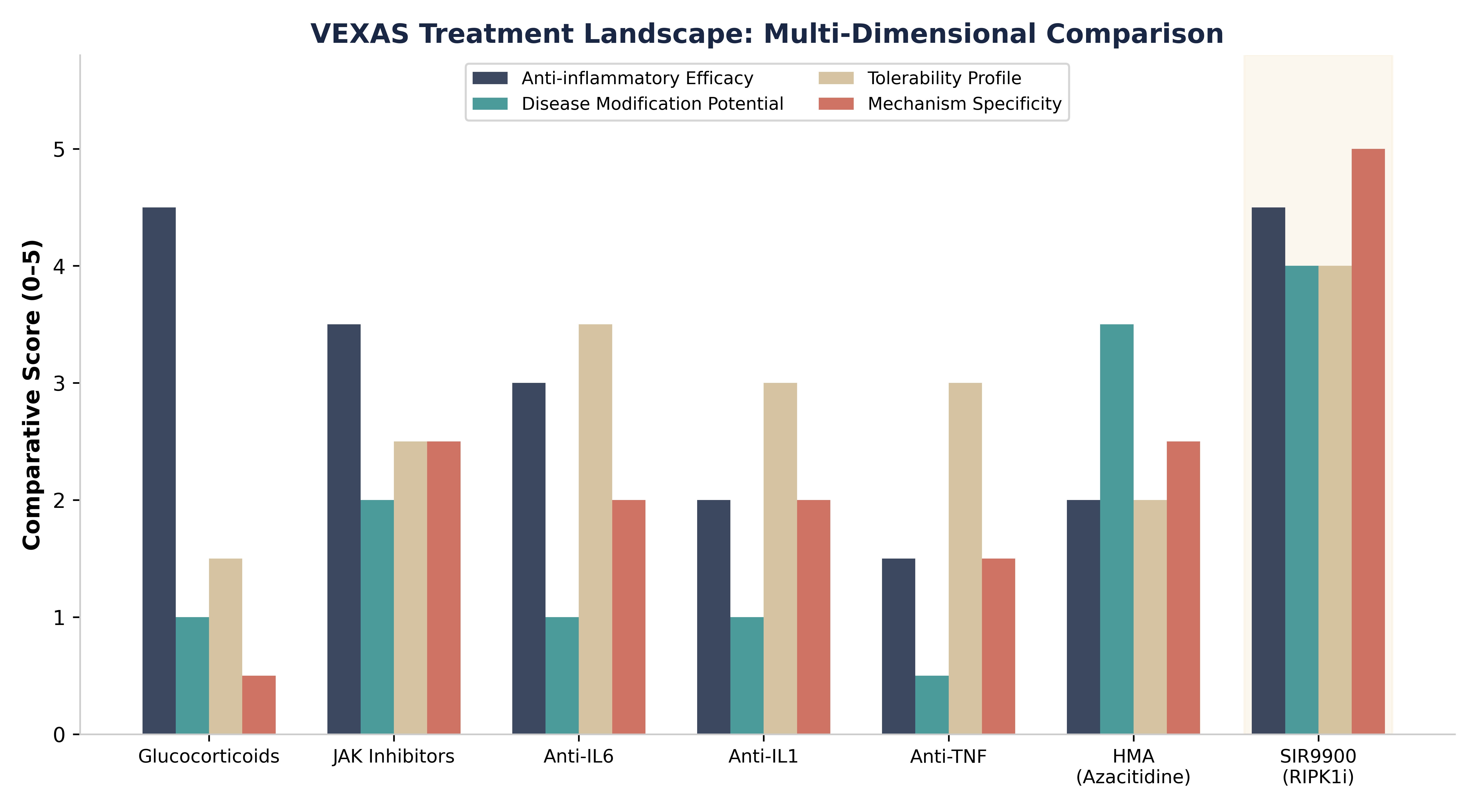
There are no FDA-approved therapies for VEXAS syndrome. Current standard of care relies on chronic glucocorticoids with significant toxicity, treatment resistance, and flare recurrence. SIR9900 represents the first mechanism-targeted therapy designed to address the proximal molecular driver of VEXAS-associated inflammation.
8 Scientific Rationale: RIPK1 in VEXAS
8.1 The RIPK1-Mediated Cell Death Axis
Recent publications have established RIPK1 kinase activity as a central driver of VEXAS autoinflammation:
Narendra et al. (Nature 2025): Demonstrated that UBA1 mutations drive RIPK1-dependent inflammatory cell death through two independent mechanisms — macrophage-driven inflammation (RIPK3-Caspase-8 pathway) and HSPC dysfunction (unfolded protein response)
Kosmider et al. (Nat Commun 2024): Showed VEXAS is characterized by inflammasome activation and monocyte dysregulation, with LDH levels correlating with RIPK1/RIPK3 activity
Breillat et al. (bioRxiv 2025): Confirmed that UBA1 mutations drive RIPK1-mediated cell death and monocyte dysfunction
The pathological cascade proceeds as follows:
UBA1 Mutation → Defective ubiquitination → RIPK1 hyperactivation → Aberrant caspase-8 apoptosis & RIPK3-MLKL necroptosis → DAMP/HMGB1 release → Feed-forward myeloid-biased inflammation
8.2 Preclinical Evidence: In Vivo Survival Rescue
Show code
fig, ax = plt.subplots(figsize=(8, 5))

hours = np.array([0, 1, 2, 3, 4, 5, 6, 7, 8, 9, 10, 11, 12])
surv_vehicle = np.array([100, 100, 100, 90, 70, 50, 30, 10, 0, 0, 0, 0, 0])
surv_sir9900 = np.array([100, 100, 100, 100, 100, 100, 100, 100, 95, 90, 90, 90, 90])
surv_wt      = np.array([100, 100, 100, 100, 100, 100, 100, 100, 100, 100, 100, 100, 100])

ax.step(hours, surv_wt,      where='post', color=SLATE, lw=2,   ls='--', label='Wild-Type + Vehicle')
ax.step(hours, surv_sir9900, where='post', color=TEAL,  lw=2.5,          label='VEXAS + SIR9900 (100 mg/kg)')
ax.step(hours, surv_vehicle, where='post', color=CORAL, lw=2.5,          label='VEXAS + Vehicle')

ax.fill_between(hours, surv_vehicle, step='post', alpha=0.08, color=CORAL)
ax.fill_between(hours, surv_sir9900, step='post', alpha=0.08, color=TEAL)

ax.annotate('100% mortality\nby 9 hours', xy=(8.5, 2), fontsize=9,
            color=CORAL, fontweight='bold', ha='center')
ax.annotate('90% survival\nwith SIR9900', xy=(11, 90), fontsize=9,
            color=TEAL, fontweight='bold', ha='center',
            xytext=(9.5, 72), arrowprops=dict(arrowstyle='->', color=TEAL, lw=1.2))

ax.set_xlabel('Hours Post TNFα Challenge', fontweight='bold', fontsize=12)
ax.set_ylabel('Survival (%)', fontweight='bold', fontsize=12)
ax.set_title('Uba1-Conditional KO VEXAS Mouse Model\nTNFα-Induced Lethality Rescue by SIR9900',
             fontweight='bold', color=NAVY, fontsize=13)
ax.set_xlim(-0.2, 12.5)
(-0.2, 12.5)Show code
ax.set_ylim(-2, 105)(-2.0, 105.0)Show code
ax.legend(frameon=True, facecolor=WHITE, edgecolor='#CCCCCC', loc='center left', fontsize=9)
ax.spines['top'].set_visible(False)
ax.spines['right'].set_visible(False)
plt.tight_layout()
plt.show()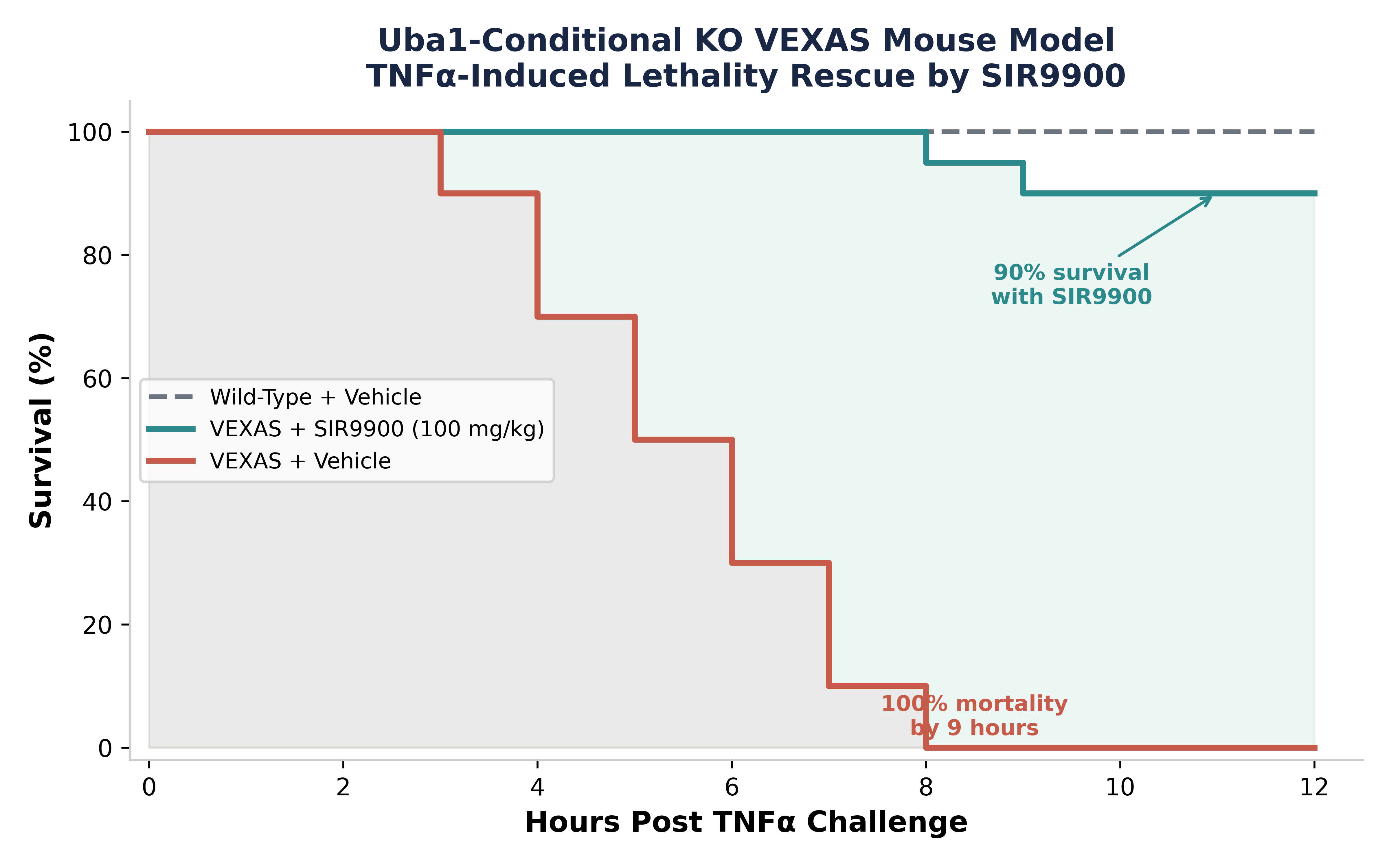
9 SIR9900: Pharmacological Profile
9.1 Target Engagement & Pharmacokinetics
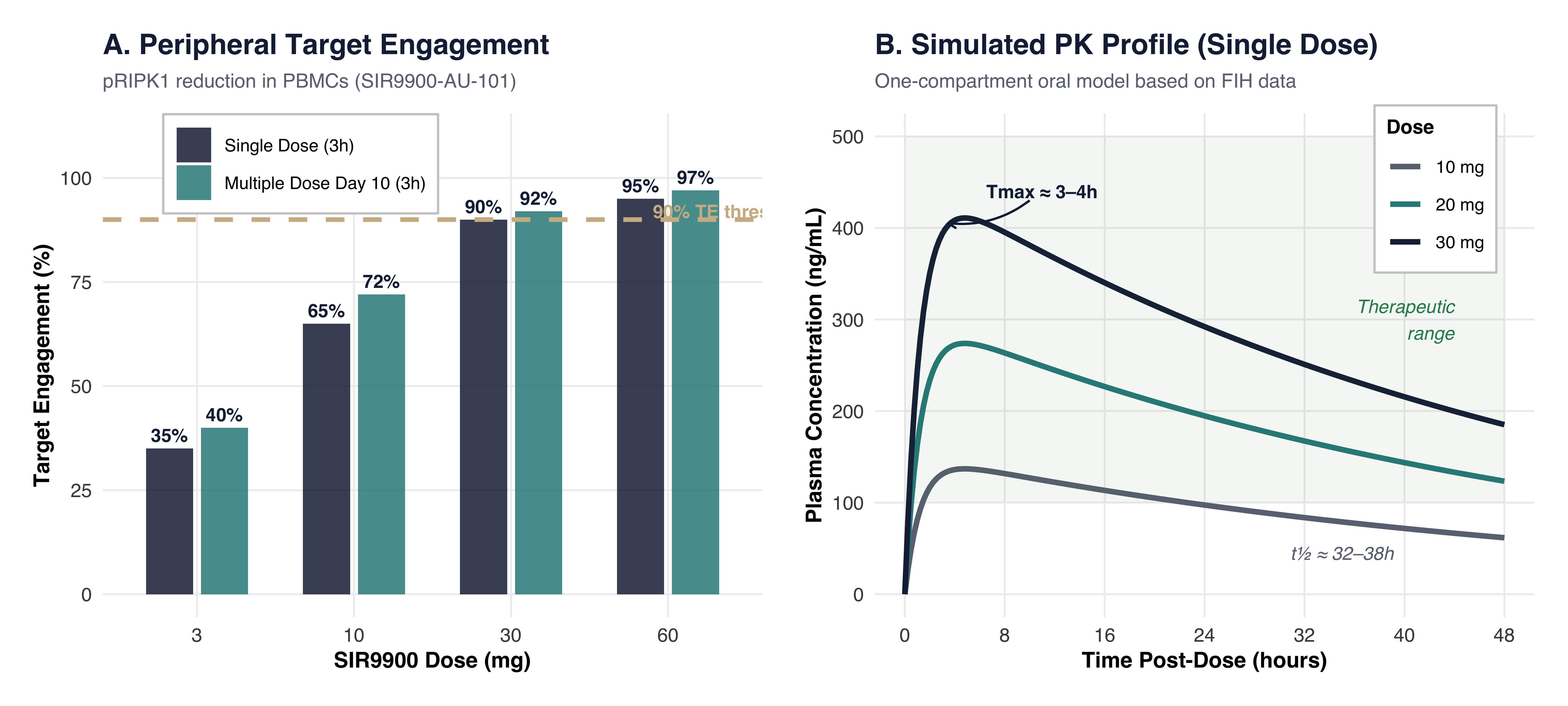
SIR9900 demonstrated robust pharmacodynamic activity in the first-in-human study (SIR9900-AU-101), achieving approximately 90% peripheral target engagement (pRIPK1 reduction in PBMCs) at 3 hours post-dose across both single and multiple dosing regimens.
Show code
library(ggplot2)
library(dplyr)
library(tidyr)
library(patchwork)
library(scales)

# ── Color palette ──
navy  <- "#1A2744"
gold  <- "#CFB991"
teal  <- "#2D8A8A"
coral <- "#C75B4A"
slate <- "#6B7280"
light_gold <- "#F5EDD8"
green_col  <- "#2D8A5E"

theme_sivex <- function(base_size = 11) {
  theme_minimal(base_size = base_size, base_family = "sans") +
    theme(
      plot.background  = element_rect(fill = "white", color = NA),
      panel.background = element_rect(fill = "white", color = NA),
      panel.grid.major = element_line(color = "#EEEEEE", linewidth = 0.4),
      panel.grid.minor = element_blank(),
      plot.title       = element_text(face = "bold", color = navy, size = 13,
                                      margin = margin(b = 6)),
      plot.subtitle    = element_text(color = slate, size = 9,
                                      margin = margin(b = 10)),
      axis.title       = element_text(face = "bold", size = 10),
      axis.text        = element_text(color = "#4A4A4A"),
      legend.position  = "bottom",
      legend.title     = element_text(face = "bold", size = 9),
      legend.text      = element_text(size = 8),
      plot.margin      = margin(10, 10, 10, 10)
    )
}

# ── Panel A: Target Engagement Bar Chart ──
te_data <- tibble(
  dose   = factor(c(3, 10, 30, 60), levels = c(3, 10, 30, 60)),
  single = c(35, 65, 90, 95),
  multi  = c(40, 72, 92, 97)
) |>
  pivot_longer(cols = c(single, multi),
               names_to = "regimen", values_to = "engagement") |>
  mutate(regimen = factor(regimen,
                          levels = c("single", "multi"),
                          labels = c("Single Dose (3h)", "Multiple Dose Day 10 (3h)")))

p1 <- ggplot(te_data, aes(x = dose, y = engagement, fill = regimen)) +
  geom_col(position = position_dodge(width = 0.7), width = 0.6, alpha = 0.85) +
  geom_text(aes(label = paste0(engagement, "%")),
            position = position_dodge(width = 0.7), vjust = -0.5,
            size = 3, fontface = "bold", color = navy) +
  geom_hline(yintercept = 90, linetype = "dashed", color = gold, linewidth = 1) +
  annotate("text", x = 4.4, y = 92, label = "90% TE threshold",
           color = gold, fontface = "bold", size = 3, hjust = 0.5) +
  scale_fill_manual(values = c(navy, teal)) +
  scale_y_continuous(limits = c(0, 110), breaks = seq(0, 100, 25)) +
  labs(
    title    = "A. Peripheral Target Engagement",
    subtitle = "pRIPK1 reduction in PBMCs (SIR9900-AU-101)",
    x = "SIR9900 Dose (mg)",
    y = "Target Engagement (%)",
    fill = NULL
  ) +
  theme_sivex() +
  theme(legend.position = c(0.3, 0.9),
        legend.background = element_rect(fill = "white", color = "#CCCCCC"))

# ── Panel B: Simulated PK Profile ──
pk_data <- expand_grid(
  dose = c(10, 20, 30),
  time = seq(0, 48, by = 0.25)
) |>
  mutate(
    ka   = 0.8,
    ke   = 0.019,
    Cmax = dose / 30 * 450,
    conc = Cmax * ka / (ka - ke) * (exp(-ke * time) - exp(-ka * time)),
    dose_label = paste0(dose, " mg")
  )

p2 <- ggplot(pk_data, aes(x = time, y = conc, color = dose_label)) +
  geom_line(linewidth = 1.2) +
  annotate("rect", xmin = 0, xmax = 48, ymin = 100, ymax = 500,
           fill = green_col, alpha = 0.06) +
  annotate("text", x = 44, y = 300, label = "Therapeutic\nrange",
           color = green_col, fontface = "italic", size = 3, hjust = 1) +
  annotate("text", x = 35, y = 45, label = "t½ ≈ 32–38h",
           color = slate, fontface = "italic", size = 3) +
  annotate("curve", x = 10, y = 430, xend = 3.5, yend = 405,
           curvature = -0.2, arrow = arrow(length = unit(0.15, "cm")),
           color = navy) +
  annotate("text", x = 11, y = 440, label = "Tmax ≈ 3–4h",
           color = navy, fontface = "bold", size = 3) +
  scale_color_manual(values = c("10 mg" = slate, "20 mg" = teal, "30 mg" = navy)) +
  scale_x_continuous(breaks = seq(0, 48, 8)) +
  labs(
    title    = "B. Simulated PK Profile (Single Dose)",
    subtitle = "One-compartment oral model based on FIH data",
    x = "Time Post-Dose (hours)",
    y = "Plasma Concentration (ng/mL)",
    color = "Dose"
  ) +
  theme_sivex() +
  theme(legend.position = c(0.85, 0.85),
        legend.background = element_rect(fill = "white", color = "#CCCCCC"))

p1 + p2 + plot_annotation(
  theme = theme(plot.background = element_rect(fill = "white", color = NA))
)
9.2 Safety Margin Analysis
SIR9900 demonstrated a favorable safety profile across nonclinical toxicology studies. The primary target organ was the testes (seminiferous tubule degeneration in rats at high doses), which was reversible upon 13 weeks of cessation.
Show code
safety_data <- tibble(
  category = c("Rat NOAEL\n(30 mg/kg/day, 26-wk)",
               "Dog NOAEL\n(150 mg/kg/day, 39-wk)",
               "Rat HED\n(4.84 mg/kg/day)",
               "Human 30 mg\n(predicted)"),
  auc      = c(110459, 450000, 110459, 8746),
  color    = c(coral, coral, teal, navy),
  type     = c("Nonclinical", "Nonclinical", "Translation", "Clinical")
) |>
  mutate(category = factor(category, levels = rev(category)))

ggplot(safety_data, aes(x = auc, y = category, fill = type)) +
  geom_col(width = 0.55, alpha = 0.85) +
  geom_text(aes(label = scales::comma(auc)),
            hjust = -0.1, fontface = "bold", size = 3.5, color = navy) +
  annotate("label", x = 300000, y = 0.7,
           label = "Safety Margin: >12.6×\n(Rat NOAEL ÷ Human 30 mg)",
           fill = light_gold, color = navy, fontface = "bold",
           size = 3.5, label.size = 0.8, label.r = unit(0.3, "lines")) +
  scale_fill_manual(values = c("Nonclinical" = coral, "Translation" = teal, "Clinical" = navy)) +
  scale_x_continuous(labels = scales::comma, limits = c(0, 530000),
                     expand = expansion(mult = c(0, 0.05))) +
  labs(
    title    = "Exposure-Based Safety Margin Analysis",
    subtitle = "AUC comparison across species and dose levels",
    x = "AUC (hr·ng/mL)",
    y = NULL,
    fill = "Category"
  ) +
  theme_sivex() +
  theme(panel.grid.major.y = element_blank(),
        legend.position = "bottom")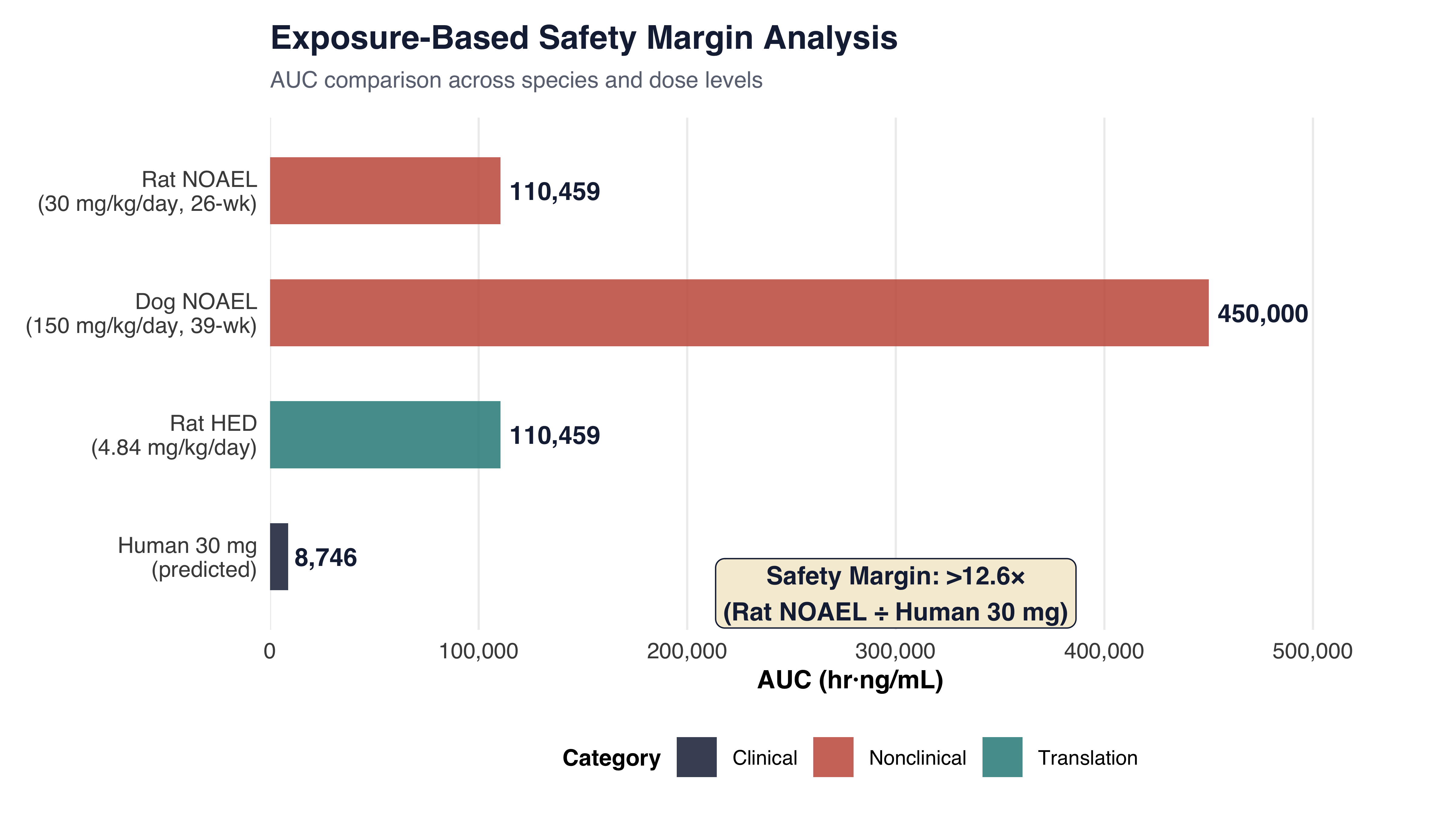
10 Study Design
10.1 Two-Part Adaptive Design
The SIVEX study employs a two-part adaptive design to efficiently identify the optimal dose and confirm efficacy:
Show code
from matplotlib.patches import FancyBboxPatch

fig, ax = plt.subplots(figsize=(10, 5.5))
ax.set_xlim(0, 10)
(0.0, 10.0)Show code
ax.set_ylim(0, 6)(0.0, 6.0)Show code
ax.axis('off')(np.float64(0.0), np.float64(10.0), np.float64(0.0), np.float64(6.0))Show code
ax.text(5, 5.7, 'SIVEX Study Schema: Two-Part Adaptive Design',
        fontsize=14, fontweight='bold', color=NAVY, ha='center', va='top')

# ── Part A ──
ax.text(0.3, 5.05, 'PART A: Dose-Ranging (N = 18–30)', fontsize=11,
        fontweight='bold', color=GOLD, va='center')

phases_a = [
    (0.3, 1.4, 'Screening\n4 wk', SLATE),
    (1.9, 2.8, 'Double-Blind\nUp to 24 wk', NAVY),
    (4.9, 2.8, 'Open-Label\n24 wk', TEAL),
    (7.9, 1.4, 'Follow-Up\n4 wk', SLATE),
]
y_a = 4.1
for x, w, label, color in phases_a:
    box = FancyBboxPatch((x, y_a), w, 0.75, boxstyle="round,pad=0.05",
                         facecolor=color, edgecolor='none', alpha=0.85)
    ax.add_patch(box)
    ax.text(x + w/2, y_a + 0.375, label, ha='center', va='center',
            fontsize=8, color='white', fontweight='bold')

arms = ['SIR9900 20 mg (N=10)', 'SIR9900 30 mg (N=10)', 'Placebo (N=10)']
for i, arm in enumerate(arms):
    yy = 3.55 - i * 0.28
    ax.text(2.3, yy, f'Arm {i+1}: {arm}', fontsize=7.5, color=NAVY)
    ax.plot([1.9, 2.2], [yy, yy], '-', color=GOLD, lw=1.5)

ax.annotate('IDMC Dose\nSelection', xy=(4.7, 4.1), xytext=(4.7, 3.15),
            fontsize=8, color=CORAL, fontweight='bold', ha='center',
            arrowprops=dict(arrowstyle='->', color=CORAL, lw=1.5))

# ── Part B ──
ax.text(0.3, 2.3, 'PART B: Efficacy & Safety (N = 80)', fontsize=11,
        fontweight='bold', color=GOLD, va='center')

y_b = 1.35
for x, w, label, color in phases_a:
    if 'Up to' in label:
        label = 'Double-Blind\n24 wk'
    box = FancyBboxPatch((x, y_b), w, 0.75, boxstyle="round,pad=0.05",
                         facecolor=color, edgecolor='none', alpha=0.85)
    ax.add_patch(box)
    ax.text(x + w/2, y_b + 0.375, label, ha='center', va='center',
            fontsize=8, color='white', fontweight='bold')

arms_b = ['SIR9900 selected dose (N=40)', 'Placebo (N=40)']
for i, arm in enumerate(arms_b):
    yy = 0.85 - i * 0.28
    ax.text(2.3, yy, f'Arm {i+1}: {arm}', fontsize=7.5, color=NAVY)
    ax.plot([1.9, 2.2], [yy, yy], '-', color=GOLD, lw=1.5)

for y_start in [y_a + 0.375, y_b + 0.375]:
    ax.annotate('', xy=(4.9, y_start), xytext=(4.7, y_start),
                arrowprops=dict(arrowstyle='->', color=GOLD, lw=1.2))

ax.text(4.8, 0.12, '↑ Flare after Wk 12 → transition to open-label',
        fontsize=7.5, color=CORAL, style='italic', ha='center')

bbox_props = dict(boxstyle="round,pad=0.3", facecolor=LIGHT_GOLD, edgecolor=GOLD, lw=1.5)
ax.text(8.6, 0.55, 'Primary Endpoint:\nOCR at Week 24', fontsize=8.5,
        fontweight='bold', color=NAVY, ha='center', va='center', bbox=bbox_props)

plt.tight_layout()
plt.show()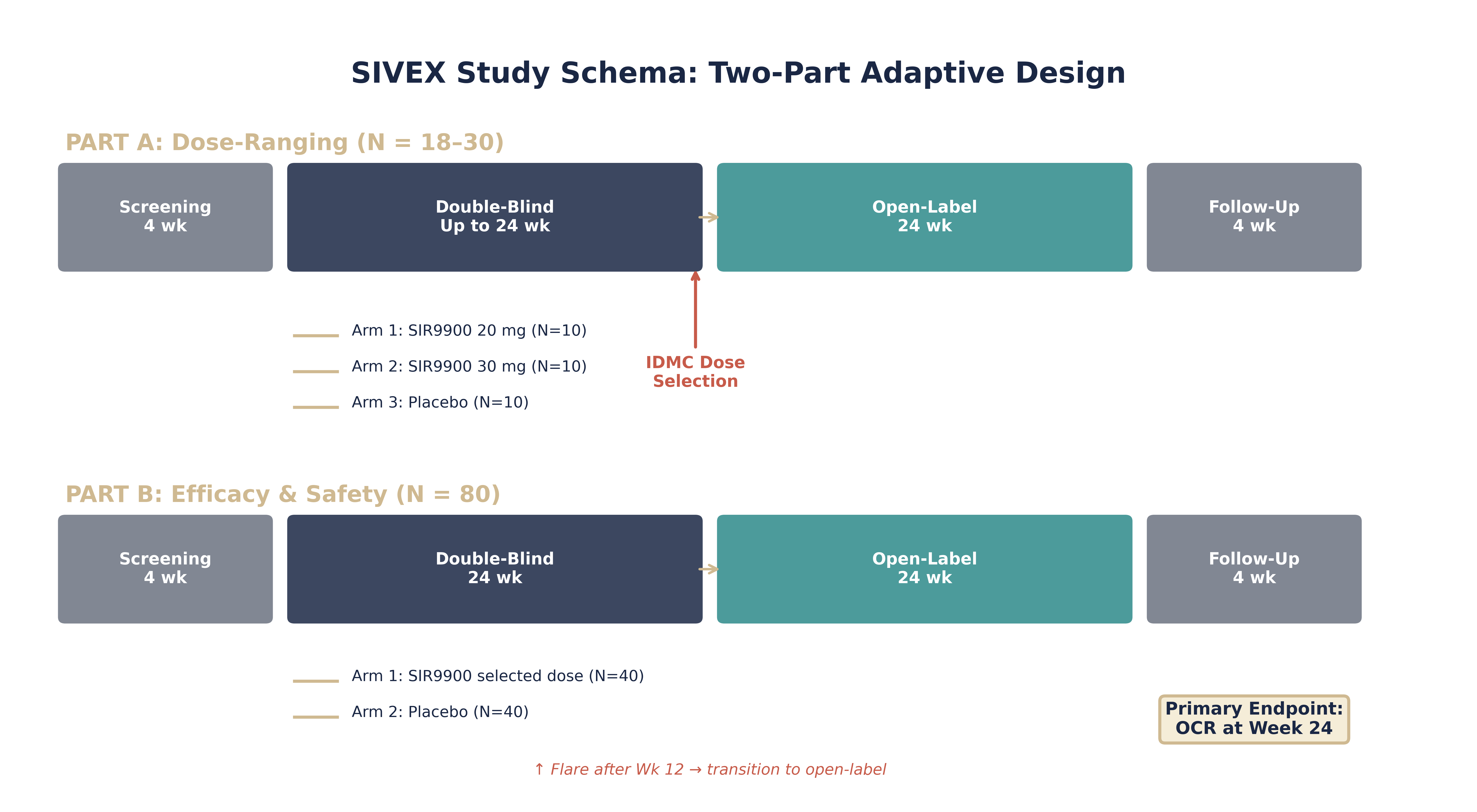
10.2 Glucocorticoid Taper Strategy
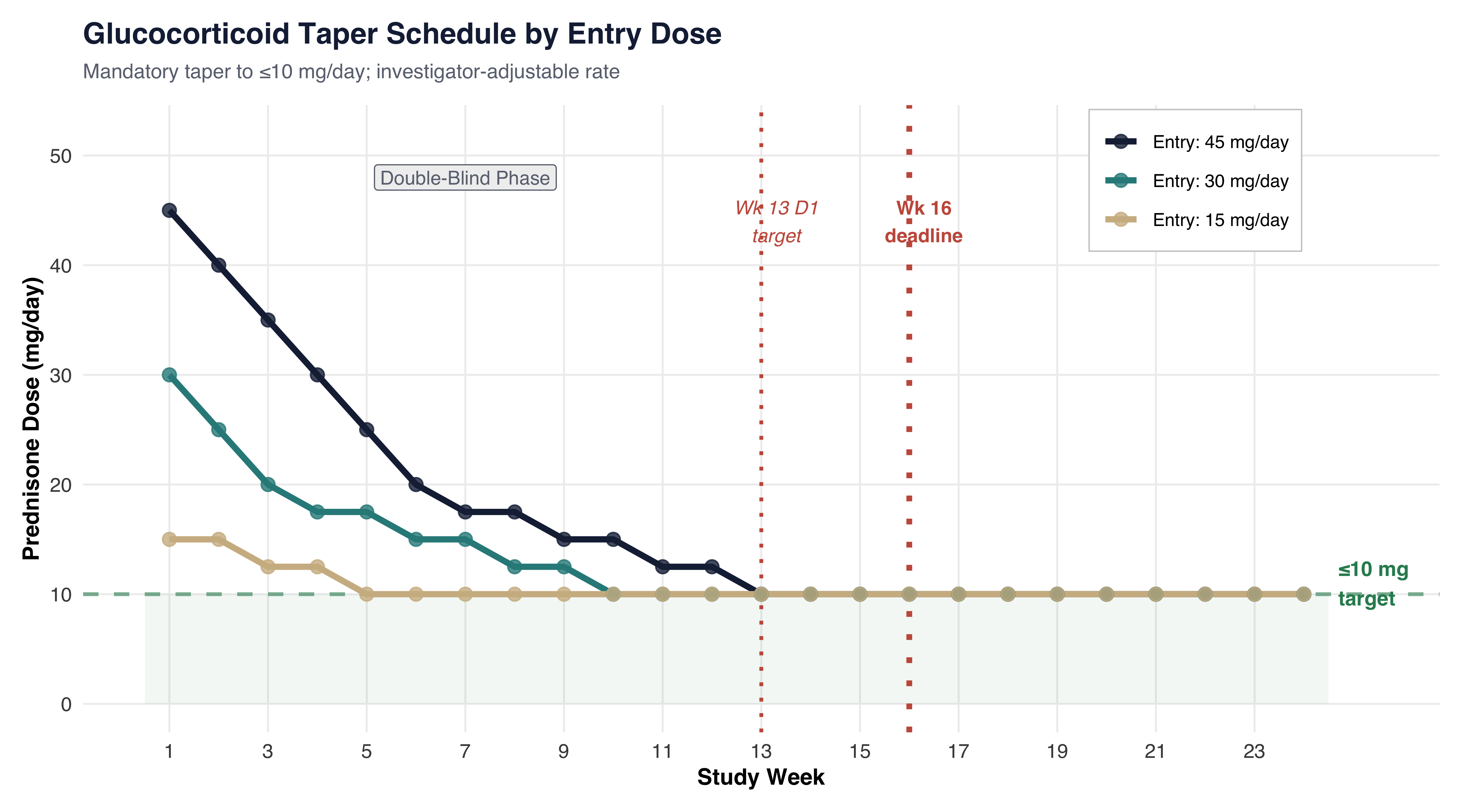
All participants undergo a mandatory glucocorticoid taper targeting ≤10 mg/day prednisone equivalent. The taper is integral to the study design — efficacy is measured by the ability to maintain flare-free status while reducing GC exposure.
Show code
taper_data <- tibble(
  week = rep(1:24, 3),
  dose = c(
    # Entry 45 mg
    45, 40, 35, 30, 25, 20, 17.5, 17.5, 15, 15, 12.5, 12.5,
    rep(10, 12),
    # Entry 30 mg
    30, 25, 20, 17.5, 17.5, 15, 15, 12.5, 12.5,
    rep(10, 15),
    # Entry 15 mg
    15, 15, 12.5, 12.5, rep(10, 20)
  ),
  entry = rep(c("Entry: 45 mg/day", "Entry: 30 mg/day", "Entry: 15 mg/day"), each = 24)
) |>
  mutate(entry = factor(entry, levels = c("Entry: 45 mg/day",
                                           "Entry: 30 mg/day",
                                           "Entry: 15 mg/day")))

ggplot(taper_data, aes(x = week, y = dose, color = entry)) +
  annotate("rect", xmin = 0.5, xmax = 24.5, ymin = 0, ymax = 10,
           fill = green_col, alpha = 0.06) +
  geom_hline(yintercept = 10, linetype = "dashed", color = green_col,
             linewidth = 0.8, alpha = 0.6) +
  geom_vline(xintercept = 13, linetype = "dotted", color = coral, linewidth = 0.8) +
  geom_vline(xintercept = 16, linetype = "dotted", color = coral, linewidth = 1.2) +
  geom_line(linewidth = 1.3) +
  geom_point(size = 2.5, alpha = 0.8) +
  annotate("text", x = 24.7, y = 11, label = "≤10 mg\ntarget",
           color = green_col, fontface = "bold", size = 3.2, hjust = 0) +
  annotate("text", x = 13.3, y = 44, label = "Wk 13 D1\ntarget",
           color = coral, fontface = "italic", size = 3) +
  annotate("text", x = 16.3, y = 44, label = "Wk 16\ndeadline",
           color = coral, fontface = "bold", size = 3) +
  annotate("label", x = 7, y = 48, label = "Double-Blind Phase",
           fill = "#F0F0F0", color = slate, size = 3, label.size = 0) +
  scale_color_manual(values = c(navy, teal, gold)) +
  scale_x_continuous(breaks = seq(1, 24, 2), limits = c(0.5, 25.5)) +
  scale_y_continuous(breaks = seq(0, 50, 10), limits = c(0, 52)) +
  labs(
    title    = "Glucocorticoid Taper Schedule by Entry Dose",
    subtitle = "Mandatory taper to ≤10 mg/day; investigator-adjustable rate",
    x = "Study Week",
    y = "Prednisone Dose (mg/day)",
    color = NULL
  ) +
  theme_sivex() +
  theme(
    legend.position = c(0.82, 0.88),
    legend.background = element_rect(fill = "white", color = "#CCCCCC",
                                     linewidth = 0.3)
  )
10.3 Overall Clinical Response Definition
The primary endpoint is the proportion of participants achieving Overall Clinical Response (OCR) by Week 24, defined as achieving clinical response or better:
| OCR? | Category | Flare-Free | GC Dose | CRP |
|---|---|---|---|---|
| YES | Stringent Clinical/Biochemical | ≥8 weeks | ≤5 mg/day | ≤10 mg/L |
| YES | Clinical/Biochemical | ≥8 weeks | ≤10 mg/day | ≤10 mg/L or ≥50%↓ to ≤20 |
| YES | Clinical Response | ≥8 weeks | ≤10 mg/day | — |
| NO | Partial Clinical | ≥8 weeks | ≥50% reduction | — |
| NO | Stable Disease | ≥8 weeks | ≤baseline dose | — |
| NO | Nonresponse | Does not meet above criteria |
A flare is defined per the consensus definition (Weeks et al. 2025) as an active inflammatory manifestation of VEXAS for which GC escalation is indicated, fulfilling ≥1 criterion from Categories A (recurrence), B (new biopsy-proven sign), or C (IAC-adjudicated manifestation).
11 Statistical Considerations
11.1 Power Analysis
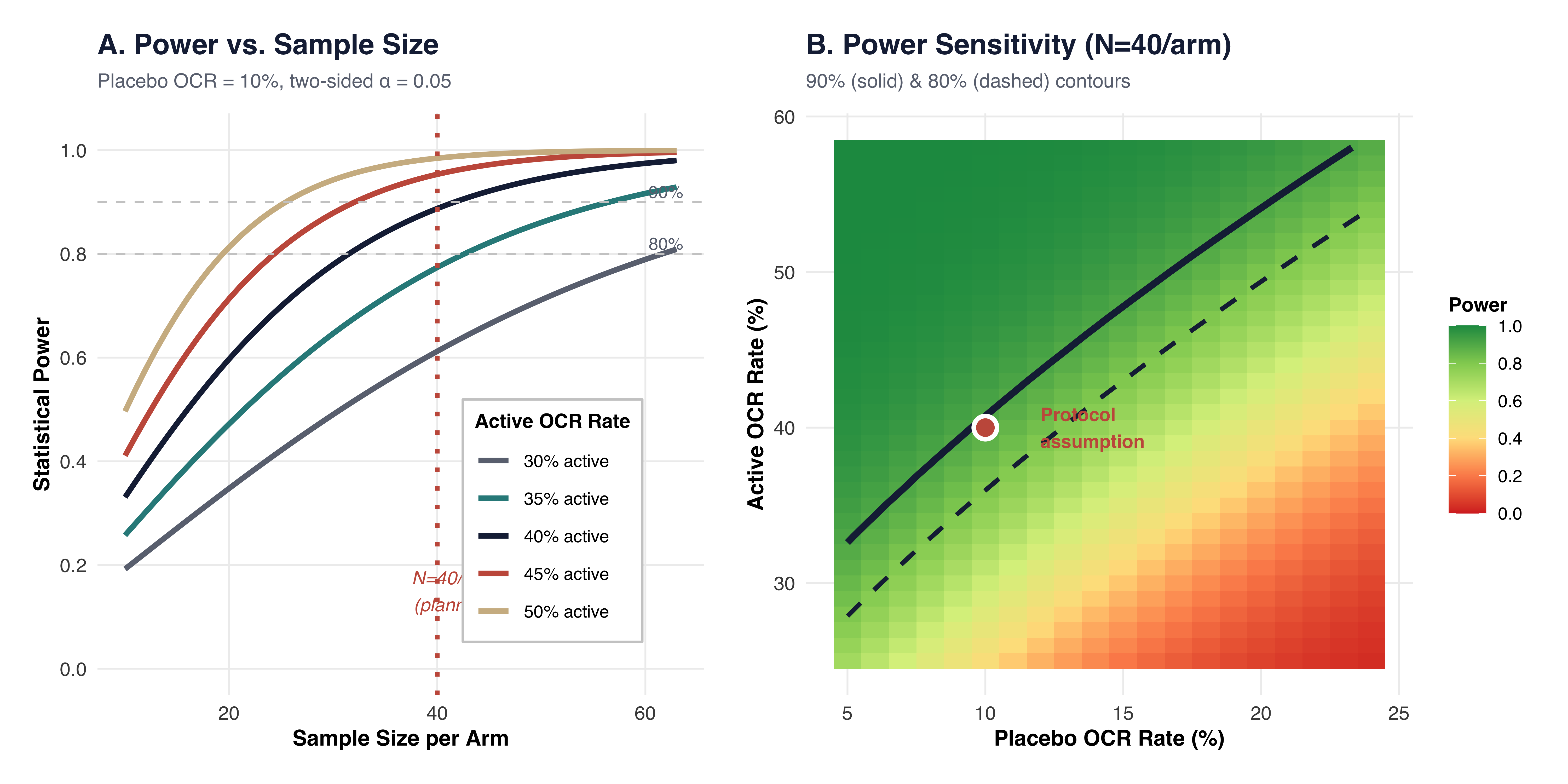
The Part B efficacy analysis assumes 40% OCR in the SIR9900 arm versus 10% in placebo, providing approximately 90% power to detect this difference using a CMH test stratified by baseline GC dose at a two-sided α = 0.05.
Show code
# ── Panel A: Power vs Sample Size ──
power_calc <- function(n, p_active, p_placebo = 0.10, alpha = 0.05) {
  p_bar  <- (p_active + p_placebo) / 2
  se_null <- sqrt(2 * p_bar * (1 - p_bar) / n)
  se_alt  <- sqrt(p_active * (1 - p_active) / n + p_placebo * (1 - p_placebo) / n)
  z_alpha <- qnorm(1 - alpha / 2)
  z <- (p_active - p_placebo - z_alpha * se_null) / se_alt
  pnorm(z)
}

power_data <- expand_grid(
  n = 10:63,
  p_active = c(0.30, 0.35, 0.40, 0.45, 0.50)
) |>
  mutate(
    power  = mapply(power_calc, n, p_active),
    active_label = paste0(p_active * 100, "% active")
  )

p_a <- ggplot(power_data, aes(x = n, y = power, color = active_label)) +
  geom_line(linewidth = 1.2) +
  geom_hline(yintercept = 0.80, linetype = "dashed", color = "#CCCCCC") +
  geom_hline(yintercept = 0.90, linetype = "dashed", color = "#CCCCCC") +
  geom_vline(xintercept = 40, linetype = "dotted", color = coral, linewidth = 1) +
  annotate("text", x = 41.5, y = 0.15, label = "N=40/arm\n(planned)",
           color = coral, fontface = "italic", size = 3) +
  annotate("text", x = 62, y = 0.82, label = "80%", color = slate, size = 2.8) +
  annotate("text", x = 62, y = 0.92, label = "90%", color = slate, size = 2.8) +
  scale_color_manual(values = c(slate, teal, navy, coral, gold)) +
  scale_y_continuous(limits = c(0, 1.02), breaks = seq(0, 1, 0.2)) +
  labs(
    title    = "A. Power vs. Sample Size",
    subtitle = "Placebo OCR = 10%, two-sided α = 0.05",
    x = "Sample Size per Arm",
    y = "Statistical Power",
    color = "Active OCR Rate"
  ) +
  theme_sivex() +
  theme(legend.position = c(0.75, 0.3),
        legend.background = element_rect(fill = "white", color = "#CCCCCC"))

# ── Panel B: Power Sensitivity Heatmap ──
sensitivity_data <- expand_grid(
  p_placebo = seq(0.05, 0.24, 0.01),
  p_active  = seq(0.25, 0.58, 0.01)
) |>
  filter(p_active > p_placebo) |>
  mutate(power = mapply(power_calc, n = 40, p_active, p_placebo))

p_b <- ggplot(sensitivity_data,
              aes(x = p_placebo * 100, y = p_active * 100, fill = power)) +
  geom_tile() +
  geom_contour(aes(z = power), breaks = 0.80,
               color = navy, linewidth = 1, linetype = "dashed") +
  geom_contour(aes(z = power), breaks = 0.90,
               color = navy, linewidth = 1.5) +
  annotate("point", x = 10, y = 40, shape = 21, size = 4,
           fill = coral, color = "white", stroke = 1.5) +
  annotate("text", x = 12, y = 40, label = "Protocol\nassumption",
           color = coral, fontface = "bold", size = 3, hjust = 0) +
  scale_fill_gradientn(
    colors = c("#D73027", "#FC8D59", "#FEE08B", "#D9EF8B", "#91CF60", "#1A9850"),
    limits = c(0, 1), breaks = seq(0, 1, 0.2),
    name = "Power"
  ) +
  labs(
    title    = "B. Power Sensitivity (N=40/arm)",
    subtitle = "90% (solid) & 80% (dashed) contours",
    x = "Placebo OCR Rate (%)",
    y = "Active OCR Rate (%)"
  ) +
  theme_sivex() +
  theme(legend.position = "right")

p_a + p_b + plot_annotation(
  theme = theme(plot.background = element_rect(fill = "white", color = NA))
)
11.2 Key Analysis Features
- Primary analysis: CMH test for OCR proportion stratified by baseline GC dose (15–25 mg vs. >25–45 mg); Full Analysis Set (ITT principle)
- Sensitivity analysis: Logistic regression with treatment, baseline GC dose, and interaction term
- Tipping point analysis: Evaluates robustness by incrementally reversing imputed responses
- Multiplicity: Gate-keeping method for 7 key secondary endpoints (tested sequentially at α=0.05)
- Subgroups: Gender, age group, prior JAK inhibitor use, baseline GC dose stratum
- Intercurrent events: Lost to follow-up, AE withdrawal, lack of efficacy → imputed as nonresponse
11.2.1 Key Secondary Endpoints (Gate-Keeping Hierarchy)
- Proportions of best response achieved (stringent clinical/biochemical → nonresponse)
- Number of flare-free days with GC ≤10 mg/day
- Cumulative glucocorticoid dose (average % of daily dose relative to baseline)
- PROMIS Physical Function 4a (T-score change from baseline)
- PROMIS Fatigue 4a (T-score change from baseline)
- Hematologic Improvement–Erythroid (HI-E) in patients with baseline Hgb <10 g/dL
- Hematologic Improvement–Platelets (HI-P) in patients with baseline PLT <100×10⁹/L
12 Projected Timeline
Show code
fig, ax = plt.subplots(figsize=(10, 4))

phases = [
    ('Regulatory / Site Activation', 2026.25, 2027.0,  SLATE),
    ('Part A: Screening',            2026.75, 2027.0,  LIGHT_GOLD),
    ('Part A: Enrollment (N ≤ 30)',   2027.0,  2027.75, NAVY),
    ('Part A: Treatment (48 wk)',     2027.0,  2028.25, TEAL),
    ('IDMC Dose Selection',           2028.0,  2028.12, CORAL),
    ('Part B: Enrollment (N = 80)',   2028.0,  2028.5,  NAVY),
    ('Part B: Treatment (48 wk)',     2028.0,  2029.25, TEAL),
    ('Part B: Follow-up & Close',     2029.25, 2029.5,  SLATE),
]

for i, (name, start, end, color) in enumerate(phases):
    width = max(end - start, 0.1)
    ax.barh(i, width, left=start, height=0.55, color=color, alpha=0.85, edgecolor='none')
    txt_color = 'white' if color in [NAVY, TEAL, CORAL, SLATE] else NAVY
    if width > 0.15:
        ax.text(start + width/2, i, name, ha='center', va='center',
                fontsize=7.5, fontweight='bold', color=txt_color)
    else:
        ax.text(end + 0.05, i, name, ha='left', va='center',
                fontsize=7.5, fontweight='bold', color=CORAL)

ax.set_yticks([])[]Show code
ax.set_xlabel('Year', fontweight='bold', fontsize=11)
ax.set_title('Projected Study Timeline', fontweight='bold', color=NAVY, fontsize=13)
ax.set_xlim(2026, 2030)
(2026.0, 2030.0)Show code
quarters = np.arange(2026, 2030.1, 0.25)
labels = []
for q in quarters:
    yr = int(q)
    qn = int((q % 1) * 4 + 1)
    labels.append(f"Q{qn}\n{yr}" if qn == 1 else f"Q{qn}")
ax.set_xticks(quarters)
ax.set_xticklabels(labels, fontsize=7)
ax.invert_yaxis()
for sp in ['top', 'right', 'left']:
    ax.spines[sp].set_visible(False)

plt.tight_layout()
plt.show()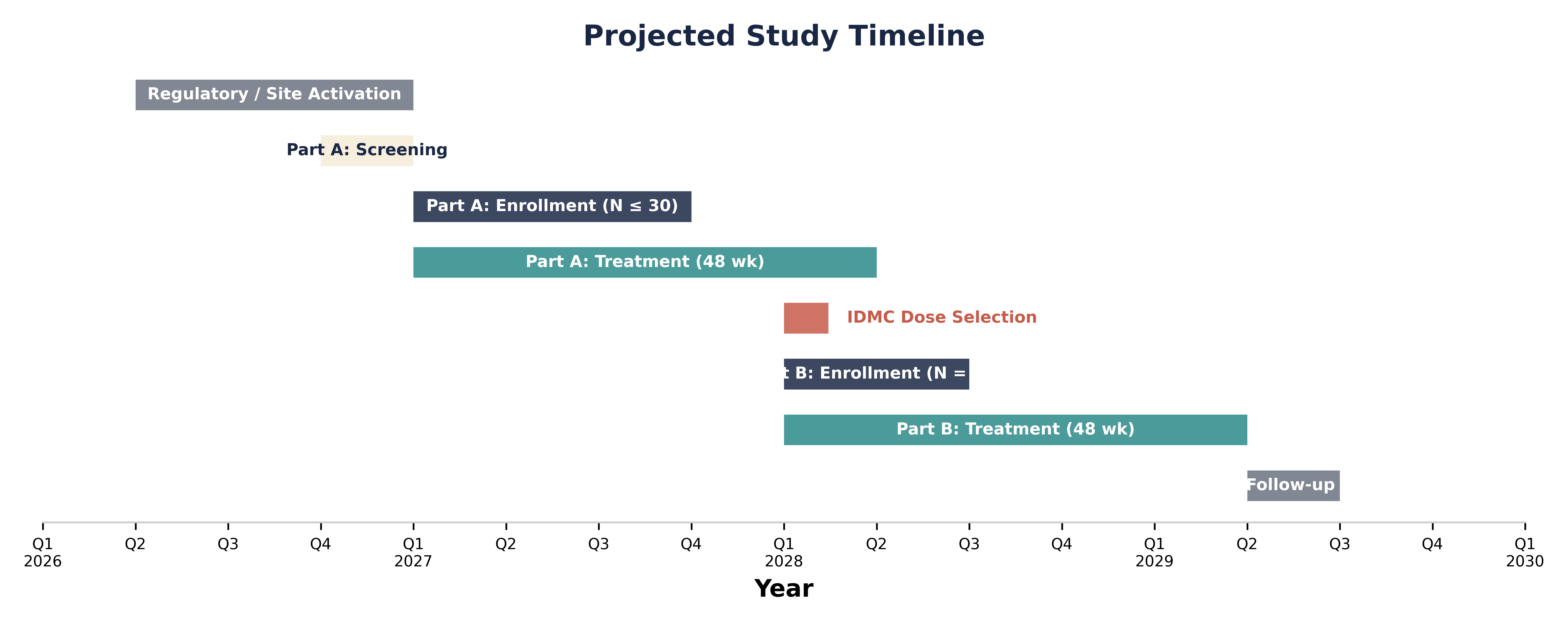
13 Eligibility Criteria Summary
13.1 Key Inclusion Criteria
- Age ≥18 years, male or female
- Documented pathogenic UBA1 mutation at M41 or splice site (c.118-1, c.118-2) by NGS, ddPCR, or Sanger sequencing
- Current or documented organ involvement within 6 months (cutaneous, vascular, musculoskeletal, ocular, periorbital, genitourinary, or pulmonary)
- Stable prednisone/prednisolone 15–45 mg/day for ≥10 days prior to enrollment
- Karnofsky Performance Status ≥50%
- Adequate organ function (AST/ALT ≤3× ULN, CrCl ≥30, ANC ≥500, PLT ≥25×10⁹/L, blasts <5%)
13.2 Key Exclusion Criteria
Prior allo-HSCT or solid organ transplant
1 ICU admission for VEXAS flare in prior 6 months
≥9 units RBC transfusion in 90 days prior
Known concurrent MDS requiring treatment or IPSS-R high/very high risk
HMA exposure within 6 months or >4 prior HMA cycles
Non-GC anti-inflammatory agents within protocol-defined washout periods (14–180 days by agent)
Strong CYP3A/CYP2C8 inhibitors/inducers or CYP1A2 substrates
Active hepatitis, uncontrolled HIV, positive QuantiFERON
14 Safety Monitoring & Oversight
14.1 Independent Committees
IDMC (Independent Data Monitoring Committee): Unblinded committee that reviews cumulative safety and efficacy data, performs dose selection in Part A, and monitors enrollment and protocol compliance.
IAC (Independent Adjudication Committee): Blinded panel of ≥3 VEXAS experts who adjudicate all suspected flares. In Part A, the IAC reviews Category C events only; in Part B, all categories (A, B, C) are adjudicated.
14.2 Adverse Event Collection
- TEAEs: Graded per CTCAE v5.0; coded by MedDRA v28.1
- Collection window: ICF signing through 28 days post last dose
- Related SAEs: Collected up to 42 days (11 half-lives)
- SAE reporting: Within 24 hours; SUSARs per regulatory timelines
15 Summary
- Strong scientific rationale: RIPK1 is validated as a central mediator of VEXAS autoinflammation by multiple independent groups; SIR9900 rescues survival in preclinical VEXAS models
- First-in-class opportunity: SIR9900 is the first RIPK1 inhibitor studied in VEXAS, targeting the proximal molecular mechanism of disease
- Robust clinical pharmacology: ~90% target engagement, favorable safety in healthy volunteers, dose-proportional PK, and >12× safety margin at the planned dose
- Rigorous Phase II design: Randomized, double-blind, placebo-controlled with adaptive dose selection, independent adjudication, and 90% statistical power
- Critical unmet need: No FDA-approved therapy exists; chronic GC dependence remains the inadequate standard of care with progressive morbidity and ~37% 5-year mortality
References
- Beck DB, et al. Somatic Mutations in UBA1 and Severe Adult-Onset Autoinflammatory Disease. N Engl J Med. 2020;383(27):2628-2638.
- Beck DB, et al. Estimated Prevalence and Clinical Manifestations of UBA1 Variants Associated With VEXAS Syndrome. JAMA. 2023;329(4):318-324.
- Narendra VK, et al. Independent mechanisms of inflammation and myeloid bias in VEXAS syndrome. Nature. 2025. doi:10.1038/s41586-025-09815-0.
- Kosmider O, et al. VEXAS syndrome is characterized by inflammasome activation and monocyte dysregulation. Nat Commun. 2024;15(1):910.
- Breillat P, et al. UBA1 Mutations Drive RIPK1-Mediated Cell Death and Monocyte Dysfunction in VEXAS Syndrome. bioRxiv. 2025.
- Georgin-Lavialle S, et al. Further characterization of clinical and laboratory features in VEXAS syndrome. Br J Dermatol. 2022;186(3):564-574.
- Weeks LD, et al. Development of a Consensus Definition of VEXAS Flare for Use in Clinical Research. ACR Convergence 2025. Poster POS1124.
- Mekinian AM, et al. ACR Guidance Statement for Diagnosis and Management of VEXAS. Arthritis Rheumatol. 2025.
Report generated: 2026-08-19 19:45:59.315956R version: R version 4.6.1 (2026-06-24)ggplot2 version: 4.0.3Python version: 3.14.0matplotlib version: 3.10.8