15  Linear regression

15.1

# Simple Linear Regression Analysis in R
# This script demonstrates the theory and implementation of simple linear regression

# Load required libraries
library(ggplot2)
library(dplyr)

Attaching package: 'dplyr'

The following objects are masked from 'package:stats':

    filter, lag

The following objects are masked from 'package:base':

    intersect, setdiff, setequal, union

library(gridExtra)

Attaching package: 'gridExtra'

The following object is masked from 'package:dplyr':

    combine

#=======================================================
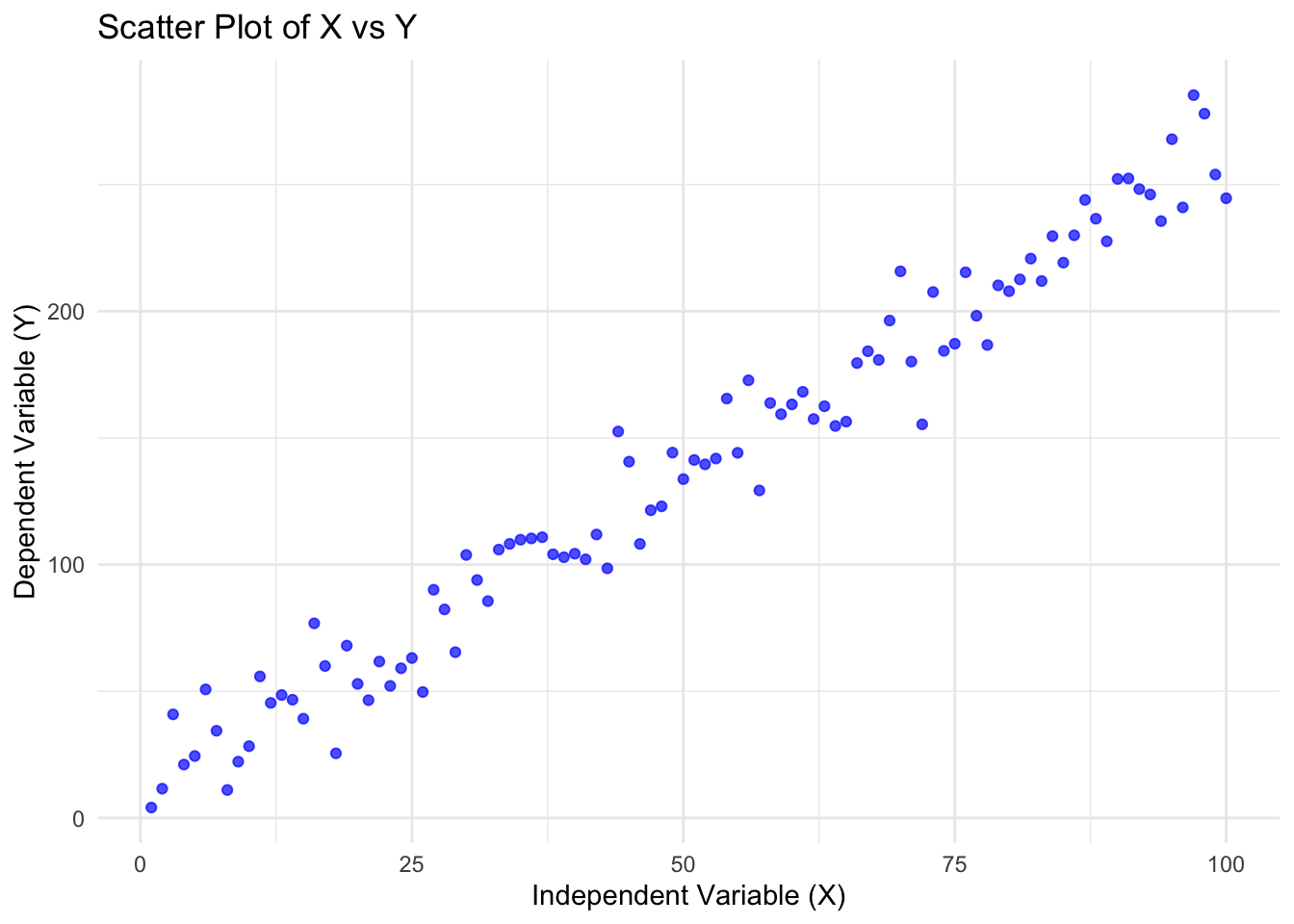
# 1. Creating a Synthetic Dataset
#=======================================================

set.seed(123) # For reproducibility
n <- 100 # Number of observations

# Independent variable (X)
x <- seq(1, 100, length.out = n)

# Create a linear relationship with some noise
true_slope <- 2.5
true_intercept <- 10
noise <- rnorm(n, mean = 0, sd = 15)
y <- true_intercept + true_slope * x + noise

# Create a dataframe
df <- data.frame(x = x, y = y)

#=======================================================
# 2. Visualizing the Data
#=======================================================

# Create a scatter plot
plt_scatter <- ggplot(df, aes(x = x, y = y)) +
  geom_point(color = "blue", alpha = 0.7) +
  labs(title = "Scatter Plot of X vs Y",
       x = "Independent Variable (X)",
       y = "Dependent Variable (Y)") +
  theme_minimal()

print(plt_scatter)

#=======================================================
# 3. Implementing Simple Linear Regression from Scratch
#=======================================================

# Manual calculation of slope and intercept using formulas
calculate_regression_params <- function(x, y) {
  n <- length(x)
  
  # Calculate means
  x_mean <- mean(x)
  y_mean <- mean(y)
  
  # Calculate slope (A)
  numerator <- sum((x - x_mean) * (y - y_mean))
  denominator <- sum((x - x_mean)^2)
  slope <- numerator / denominator
  
  # Calculate intercept (B)
  intercept <- y_mean - slope * x_mean
  
  return(list(slope = slope, intercept = intercept))
}

# Calculate parameters
params <- calculate_regression_params(df$x, df$y)
manual_slope <- params$slope
manual_intercept <- params$intercept

cat("Manually calculated parameters:\n")

Manually calculated parameters:

cat("Slope (A):", manual_slope, "\n")

Slope (A): 2.537666 

cat("Intercept (B):", manual_intercept, "\n\n")

Intercept (B): 9.453942 

# Function to make predictions
predict_y <- function(x, slope, intercept) {
  return(intercept + slope * x)
}

# Add predictions to our dataframe
df$y_pred <- predict_y(df$x, manual_slope, manual_intercept)

# Add the regression line to our scatter plot
plt_with_line <- plt_scatter +
  geom_line(data = df, aes(x = x, y = y_pred), color = "red", size = 1) +
  labs(title = "Linear Regression: Fitted Line",
       subtitle = paste("y =", round(manual_intercept, 2), "+", round(manual_slope, 2), "* x"))

Warning: Using `size` aesthetic for lines was deprecated in ggplot2 3.4.0.
ℹ Please use `linewidth` instead.

print(plt_with_line)

#=======================================================
# 4. Calculating Residuals and Error Metrics
#=======================================================

# Calculate residuals
df$residuals <- df$y - df$y_pred

# Calculate Mean Squared Error (MSE)
mse <- mean(df$residuals^2)

# Calculate Root Mean Squared Error (RMSE)
rmse <- sqrt(mse)

# Calculate R-squared
y_mean <- mean(df$y)
ss_total <- sum((df$y - y_mean)^2)
ss_residual <- sum(df$residuals^2)
r_squared <- 1 - (ss_residual / ss_total)

cat("Error Metrics:\n")

Error Metrics:

cat("Mean Squared Error (MSE):", mse, "\n")

Mean Squared Error (MSE): 184.4204 

cat("Root Mean Squared Error (RMSE):", rmse, "\n")

Root Mean Squared Error (RMSE): 13.58015 

cat("R-squared (R²):", r_squared, "\n\n")

R-squared (R²): 0.9667731 

#=======================================================
# 5. Implementing Gradient Descent for Linear Regression
#=======================================================

gradient_descent <- function(x, y, learning_rate = 0.0001, iterations = 1000) {
  # Initialize parameters
  slope <- 0
  intercept <- 0
  n <- length(x)
  
  # Storage for tracking
  mse_history <- numeric(iterations)
  slope_history <- numeric(iterations)
  intercept_history <- numeric(iterations)
  
  # Normalize x to avoid potential numerical issues
  x_scaled <- scale(x)
  x_mean <- attr(x_scaled, "scaled:center")
  x_sd <- attr(x_scaled, "scaled:scale")
  x_scaled <- as.vector(x_scaled)
  
  for (i in 1:iterations) {
    # Predict with current parameters
    y_pred <- intercept + slope * x_scaled
    
    # Calculate gradients
    grad_intercept <- -2/n * sum(y - y_pred)
    grad_slope <- -2/n * sum(x_scaled * (y - y_pred))
    
    # Update parameters
    intercept <- intercept - learning_rate * grad_intercept
    slope <- slope - learning_rate * grad_slope
    
    # Store current values
    slope_history[i] <- slope
    intercept_history[i] <- intercept
    mse_history[i] <- mean((y - (intercept + slope * x_scaled))^2)
  }
  
  # Convert slope back to original scale
  slope_original <- slope / x_sd
  intercept_original <- intercept - slope * x_mean / x_sd
  
  return(list(
    slope = slope_original, 
    intercept = intercept_original,
    mse_history = mse_history,
    slope_history = slope_history,
    intercept_history = intercept_history
  ))
}

# Run gradient descent
gd_results <- gradient_descent(df$x, df$y, learning_rate = 0.00001, iterations = 1000)

cat("Gradient Descent Results:\n")

Gradient Descent Results:

cat("Slope (A):", gd_results$slope, "\n")

Slope (A): 0.04975211 

cat("Intercept (B):", gd_results$intercept, "\n\n")

Intercept (B): 0.2123284 

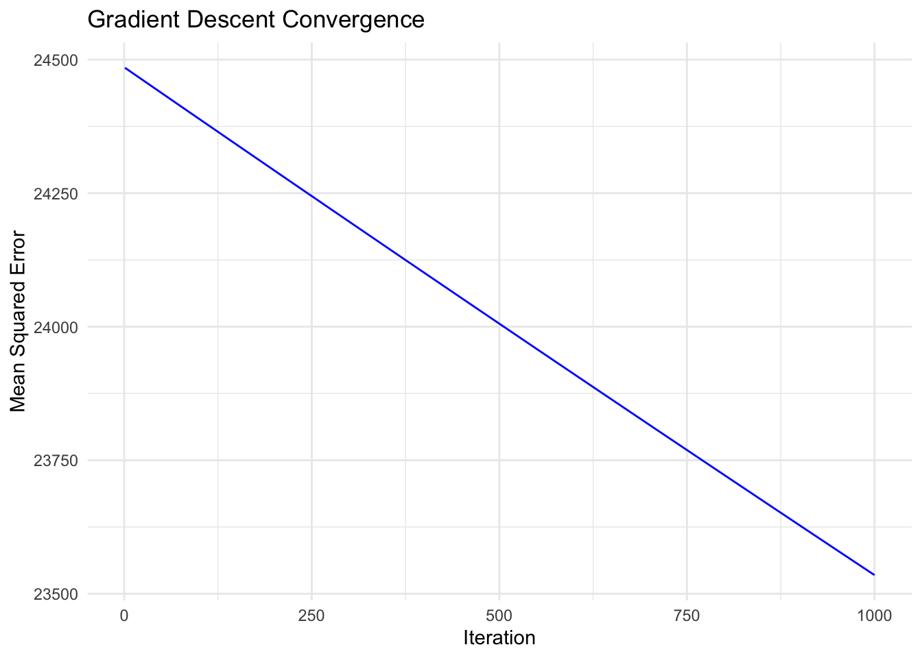
# Plot MSE history to show convergence
plt_mse <- ggplot(data.frame(iteration = 1:1000, mse = gd_results$mse_history), 
                 aes(x = iteration, y = mse)) +
  geom_line(color = "blue") +
  labs(title = "Gradient Descent Convergence",
       x = "Iteration",
       y = "Mean Squared Error") +
  theme_minimal()

print(plt_mse)

#=======================================================
# 6. Using Built-in R Function for Linear Regression
#=======================================================

# Fit a linear model using lm()
lm_model <- lm(y ~ x, data = df)

# Print summary
cat("Linear Model Summary:\n")

Linear Model Summary:

print(summary(lm_model))

Call:
lm(formula = y ~ x, data = df)

Residuals:
    Min      1Q  Median      3Q     Max 
-36.803  -8.285  -0.519   9.727  31.423 

Coefficients:
            Estimate Std. Error t value Pr(>|t|)    
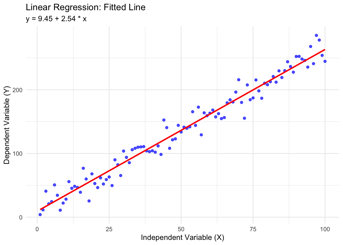
(Intercept)  9.45394    2.76431    3.42 0.000914 ***
x            2.53767    0.04752   53.40  < 2e-16 ***
---
Signif. codes:  0 '***' 0.001 '**' 0.01 '*' 0.05 '.' 0.1 ' ' 1

Residual standard error: 13.72 on 98 degrees of freedom
Multiple R-squared:  0.9668,    Adjusted R-squared:  0.9664 
F-statistic:  2851 on 1 and 98 DF,  p-value: < 2.2e-16

# Get coefficients
lm_intercept <- coef(lm_model)[1]
lm_slope <- coef(lm_model)[2]

cat("\nComparing all methods:\n")

Comparing all methods:

cat("True parameters: Slope =", true_slope, "Intercept =", true_intercept, "\n")

True parameters: Slope = 2.5 Intercept = 10 

cat("Manual calculation: Slope =", round(manual_slope, 4), "Intercept =", round(manual_intercept, 4), "\n")

Manual calculation: Slope = 2.5377 Intercept = 9.4539 

cat("Gradient descent: Slope =", round(gd_results$slope, 4), "Intercept =", round(gd_results$intercept, 4), "\n")

Gradient descent: Slope = 0.0498 Intercept = 0.2123 

cat("lm() function: Slope =", round(lm_slope, 4), "Intercept =", round(lm_intercept, 4), "\n\n")

lm() function: Slope = 2.5377 Intercept = 9.4539 

#=======================================================
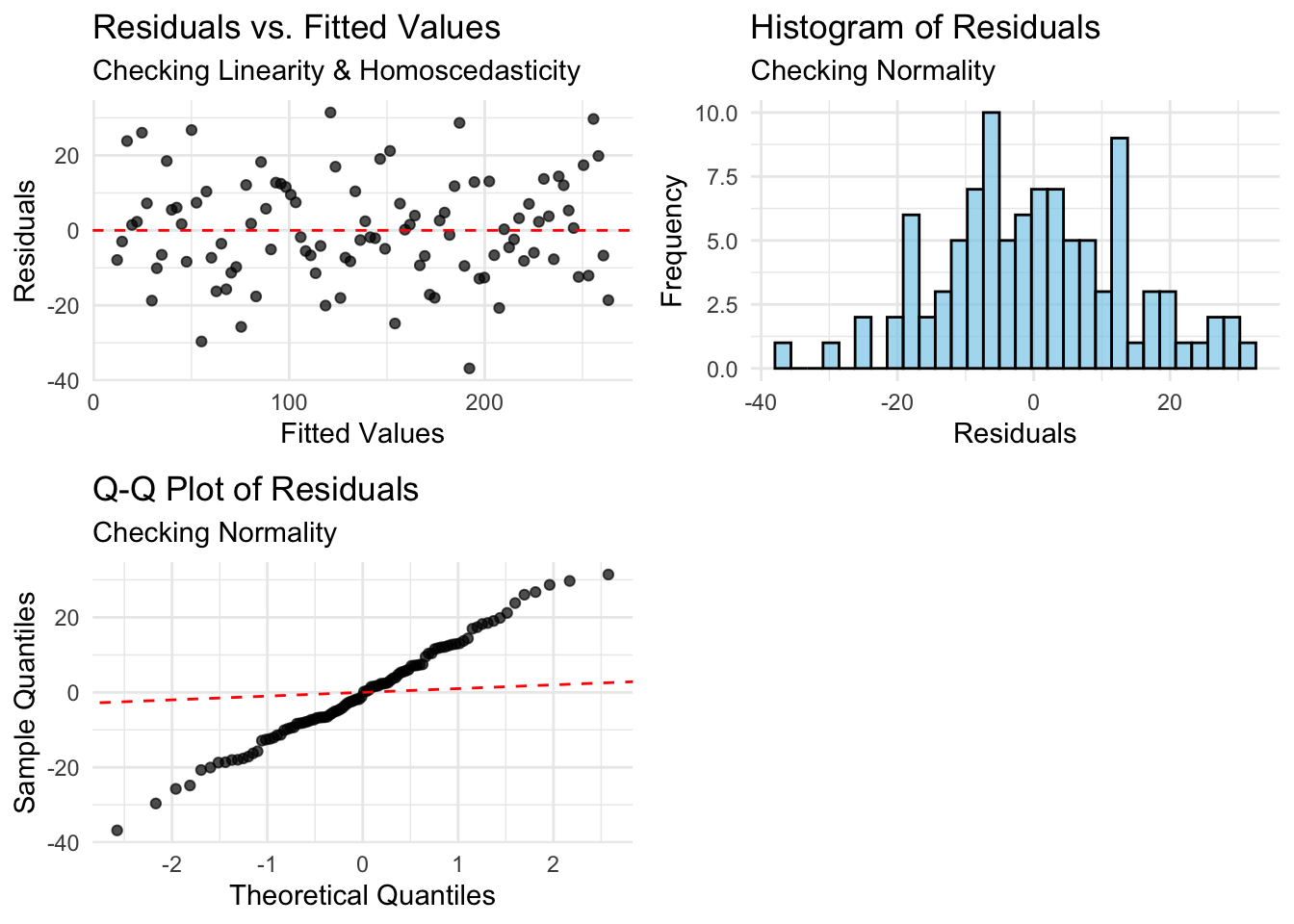
# 7. Checking Linear Regression Assumptions
#=======================================================

# 1. Linearity: Create residual vs. fitted plot
plt_residuals_fitted <- ggplot(data.frame(fitted = fitted(lm_model), 
                                         residuals = residuals(lm_model)), 
                              aes(x = fitted, y = residuals)) +
  geom_point(alpha = 0.7) +
  geom_hline(yintercept = 0, linetype = "dashed", color = "red") +
  labs(title = "Residuals vs. Fitted Values",
       subtitle = "Checking Linearity & Homoscedasticity",
       x = "Fitted Values",
       y = "Residuals") +
  theme_minimal()

# 2. Normality of residuals: Create a histogram and QQ plot
plt_hist <- ggplot(data.frame(residuals = residuals(lm_model)), aes(x = residuals)) +
  geom_histogram(bins = 30, fill = "skyblue", color = "black", alpha = 0.7) +
  labs(title = "Histogram of Residuals",
       subtitle = "Checking Normality",
       x = "Residuals",
       y = "Frequency") +
  theme_minimal()

# Create QQ plot data
qq_data <- data.frame(
  theoretical = qnorm(ppoints(length(residuals(lm_model)))),
  sample = sort(residuals(lm_model))
)

plt_qq <- ggplot(qq_data, aes(x = theoretical, y = sample)) +
  geom_point(alpha = 0.7) +
  geom_abline(intercept = 0, slope = 1, color = "red", linetype = "dashed") +
  labs(title = "Q-Q Plot of Residuals",
       subtitle = "Checking Normality",
       x = "Theoretical Quantiles",
       y = "Sample Quantiles") +
  theme_minimal()

# 3. Independence: Not easily testable with a plot for this simple data
# 4. Homoscedasticity: Already covered in residuals vs. fitted plot

# Display diagnostic plots
grid.arrange(plt_residuals_fitted, plt_hist, plt_qq, ncol = 2)

#=======================================================
# 8. Making Predictions with the Model
#=======================================================

# Create new data for prediction
new_x <- data.frame(x = c(25, 50, 75))

# Predict using the model
new_x$predicted_y <- predict(lm_model, newdata = new_x)

cat("Predictions for new data:\n")

Predictions for new data:

print(new_x)

   x predicted_y
1 25     72.8956
2 50    136.3373
3 75    199.7789

# Add prediction intervals
predictions_with_intervals <- predict(lm_model, newdata = new_x, interval = "prediction", level = 0.95)
new_x_with_intervals <- cbind(new_x, predictions_with_intervals)

cat("\nPredictions with 95% prediction intervals:\n")

Predictions with 95% prediction intervals:

print(new_x_with_intervals)

   x predicted_y      fit       lwr      upr
1 25     72.8956  72.8956  45.43136 100.3598
2 50    136.3373 136.3373 108.97847 163.6960
3 75    199.7789 199.7789 172.32277 227.2350

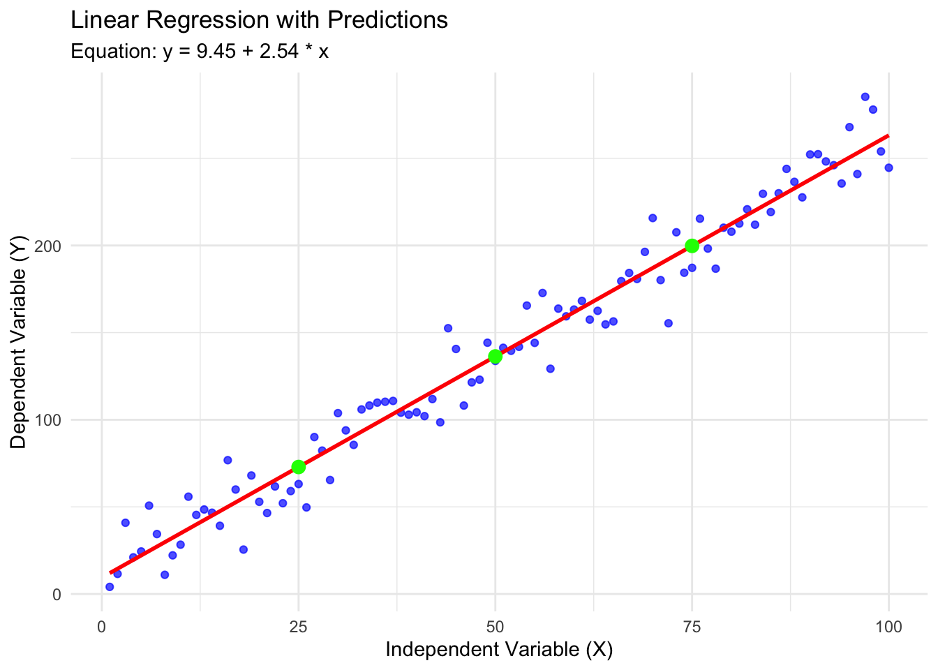
# Visualize predictions on the original plot
plt_predictions <- plt_with_line +
  geom_point(data = new_x, aes(x = x, y = predicted_y), color = "green", size = 3) +
  labs(title = "Linear Regression with Predictions",
       subtitle = paste("Equation: y =", round(lm_intercept, 2), "+", round(lm_slope, 2), "* x"))

print(plt_predictions)

#=======================================================
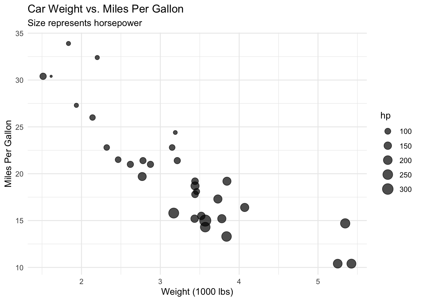
# 9. Real-World Example: Car MPG vs. Weight
#=======================================================

# Load the mtcars dataset
data(mtcars)

# Create a scatter plot
plt_cars <- ggplot(mtcars, aes(x = wt, y = mpg)) +
  geom_point(aes(size = hp), alpha = 0.7) +
  labs(title = "Car Weight vs. Miles Per Gallon",
       subtitle = "Size represents horsepower",
       x = "Weight (1000 lbs)",
       y = "Miles Per Gallon") +
  theme_minimal()

print(plt_cars)

# Fit a linear model
car_model <- lm(mpg ~ wt, data = mtcars)

# Print summary
cat("\nCar Model Summary:\n")

Car Model Summary:

print(summary(car_model))

Call:
lm(formula = mpg ~ wt, data = mtcars)

Residuals:
    Min      1Q  Median      3Q     Max 
-4.5432 -2.3647 -0.1252  1.4096  6.8727 

Coefficients:
            Estimate Std. Error t value Pr(>|t|)    
(Intercept)  37.2851     1.8776  19.858  < 2e-16 ***
wt           -5.3445     0.5591  -9.559 1.29e-10 ***
---
Signif. codes:  0 '***' 0.001 '**' 0.01 '*' 0.05 '.' 0.1 ' ' 1

Residual standard error: 3.046 on 30 degrees of freedom
Multiple R-squared:  0.7528,    Adjusted R-squared:  0.7446 
F-statistic: 91.38 on 1 and 30 DF,  p-value: 1.294e-10

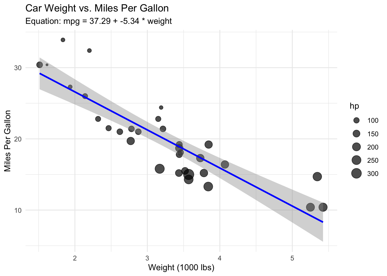
# Add regression line to the plot
plt_cars_with_line <- plt_cars +
  geom_smooth(method = "lm", se = TRUE, color = "blue") +
  labs(subtitle = paste("Equation: mpg =", round(coef(car_model)[1], 2), 
                        "+", round(coef(car_model)[2], 2), "* weight"))

print(plt_cars_with_line)

`geom_smooth()` using formula = 'y ~ x'

# Create a prediction function
predict_mpg <- function(weight) {
  return(coef(car_model)[1] + coef(car_model)[2] * weight)
}

# Example prediction
new_weight <- 3.5  # 3,500 lbs
predicted_mpg <- predict_mpg(new_weight)
cat("\nPredicted MPG for a car weighing", new_weight * 1000, "lbs:", round(predicted_mpg, 2))

Predicted MPG for a car weighing 3500 lbs: 18.58

15.2 Regression vs Stratifcation vs Matching

# Load necessary libraries
library(ggplot2)
library(dplyr)
library(MatchIt)
library(broom)

# Set seed for reproducibility
set.seed(123)

#-------------------------------------------------------------------------
# Create a simulated dataset for our examples
#-------------------------------------------------------------------------
# Sample size
n <- 500

# Simulate age (older patients more likely to get treatment B)
age <- rnorm(n, mean = 50, sd = 10)

# Simulate sex (binary for simplicity)
sex <- rbinom(n, 1, 0.5)

# Treatment assignment depends on age (older patients more likely to get B)
# and sex (females more likely to get B)
p_treatment_B <- plogis(-3 + 0.05 * age + 0.8 * sex)
treatment <- rbinom(n, 1, p_treatment_B)
treatment_label <- ifelse(treatment == 1, "B", "A")

# True treatment effect is 2
true_effect <- 2

# Outcome depends on treatment, age, and sex
# Age has a non-linear effect
outcome <- 10 + true_effect * treatment + 0.2 * age + 2 * sex + 0.01 * age^2 + rnorm(n, 0, 5)

# Create the dataset
data <- data.frame(
  patient_id = 1:n,
  age = age,
  sex = factor(sex, labels = c("Male", "Female")),
  treatment = factor(treatment_label, levels = c("A", "B")),
  outcome = outcome
)

#-------------------------------------------------------------------------
# 1. Simple regression without adjustment
#-------------------------------------------------------------------------
model_unadjusted <- lm(outcome ~ treatment, data = data)
summary_unadjusted <- summary(model_unadjusted)

cat("Unadjusted Treatment Effect:\n")

Unadjusted Treatment Effect:

print(coef(summary_unadjusted)["treatmentB", ])

    Estimate   Std. Error      t value     Pr(>|t|) 
8.030098e+00 1.154821e+00 6.953543e+00 1.123572e-11 

#-------------------------------------------------------------------------
# 2. Regression with adjustment for sex and age
#-------------------------------------------------------------------------
model_adjusted <- lm(outcome ~ treatment + sex + age, data = data)
summary_adjusted <- summary(model_adjusted)

cat("\nAdjusted Treatment Effect (linear adjustment for age):\n")

Adjusted Treatment Effect (linear adjustment for age):

print(coef(summary_adjusted)["treatmentB", ])

    Estimate   Std. Error      t value     Pr(>|t|) 
2.290267e+00 4.807315e-01 4.764130e+00 2.494562e-06 

# Check for non-linear age effect
model_nonlinear <- lm(outcome ~ treatment + sex + age + I(age^2), data = data)
summary_nonlinear <- summary(model_nonlinear)

cat("\nTesting if non-linear age adjustment improves model:\n")

Testing if non-linear age adjustment improves model:

anova(model_adjusted, model_nonlinear)

Analysis of Variance Table

Model 1: outcome ~ treatment + sex + age
Model 2: outcome ~ treatment + sex + age + I(age^2)
  Res.Df   RSS Df Sum of Sq      F    Pr(>F)    
1    496 12987                                  
2    495 12246  1     740.6 29.935 7.106e-08 ***
---
Signif. codes:  0 '***' 0.001 '**' 0.01 '*' 0.05 '.' 0.1 ' ' 1

#-------------------------------------------------------------------------
# 3. Stratification approach by sex
#-------------------------------------------------------------------------
# Compute treatment effect within each sex
strat_by_sex <- data %>%
  group_by(sex) %>%
  do(model = lm(outcome ~ treatment, data = .)) %>%
  mutate(treatment_effect = coef(model)["treatmentB"])

cat("\nStratified Treatment Effects by Sex:\n")

Stratified Treatment Effects by Sex:

print(strat_by_sex[, c("sex", "treatment_effect")])

# A tibble: 2 × 2
# Rowwise: 
  sex    treatment_effect
  <fct>             <dbl>
1 Male               7.71
2 Female             7.60

# Average of stratified effects
avg_strat_effect_sex <- mean(strat_by_sex$treatment_effect)
cat("\nAverage of sex-stratified treatment effects:", avg_strat_effect_sex, "\n")

Average of sex-stratified treatment effects: 7.652672 

#-------------------------------------------------------------------------
# 4. Stratification approach by age quintiles
#-------------------------------------------------------------------------
# Create age quintiles
data$age_quintile <- cut(data$age, 
                         breaks = quantile(data$age, probs = seq(0, 1, 0.2)),
                         labels = paste0("Q", 1:5),
                         include.lowest = TRUE)

# Compute treatment effect within each age quintile
strat_by_age <- data %>%
  group_by(age_quintile) %>%
  do(model = lm(outcome ~ treatment, data = .)) %>%
  mutate(treatment_effect = coef(model)["treatmentB"],
         n_patients = sum(!is.na(model$model$outcome)))

cat("\nStratified Treatment Effects by Age Quintile:\n")

Stratified Treatment Effects by Age Quintile:

print(strat_by_age[, c("age_quintile", "treatment_effect", "n_patients")])

# A tibble: 5 × 3
# Rowwise: 
  age_quintile treatment_effect n_patients
  <fct>                   <dbl>      <int>
1 Q1                       1.48        100
2 Q2                       3.50        100
3 Q3                       1.77        100
4 Q4                       2.44        100
5 Q5                       7.55        100

# Average of stratified effects
avg_strat_effect_age <- mean(strat_by_age$treatment_effect)
cat("\nAverage of age-quintile-stratified treatment effects:", avg_strat_effect_age, "\n")

Average of age-quintile-stratified treatment effects: 3.348508 

#-------------------------------------------------------------------------
# 5. Matching approach - FIXED VERSION
#-------------------------------------------------------------------------
# Match on age (within 2 years)
# Fix: When using mahalanobis distance, caliper must be named
m_out <- matchit(treatment == "B" ~ age, 
                 data = data,
                 method = "nearest", 
                 distance = "mahalanobis",
                 caliper = c(age = 2/sd(data$age)))  # Named caliper for age

# Get matched data
matched_data <- match.data(m_out)

# Analyze matched data
matched_model <- lm(outcome ~ treatment, data = matched_data, weights = weights)
summary_matched <- summary(matched_model)

cat("\nMatched Analysis Treatment Effect:\n")

Matched Analysis Treatment Effect:

print(coef(summary_matched)["treatmentB", ])

  Estimate Std. Error    t value   Pr(>|t|) 
2.52506949 1.15911806 2.17844031 0.02995363 

cat("Number of matched pairs:", m_out$nn["Matched", "Control"], "\n")

Number of matched pairs: 

#-------------------------------------------------------------------------
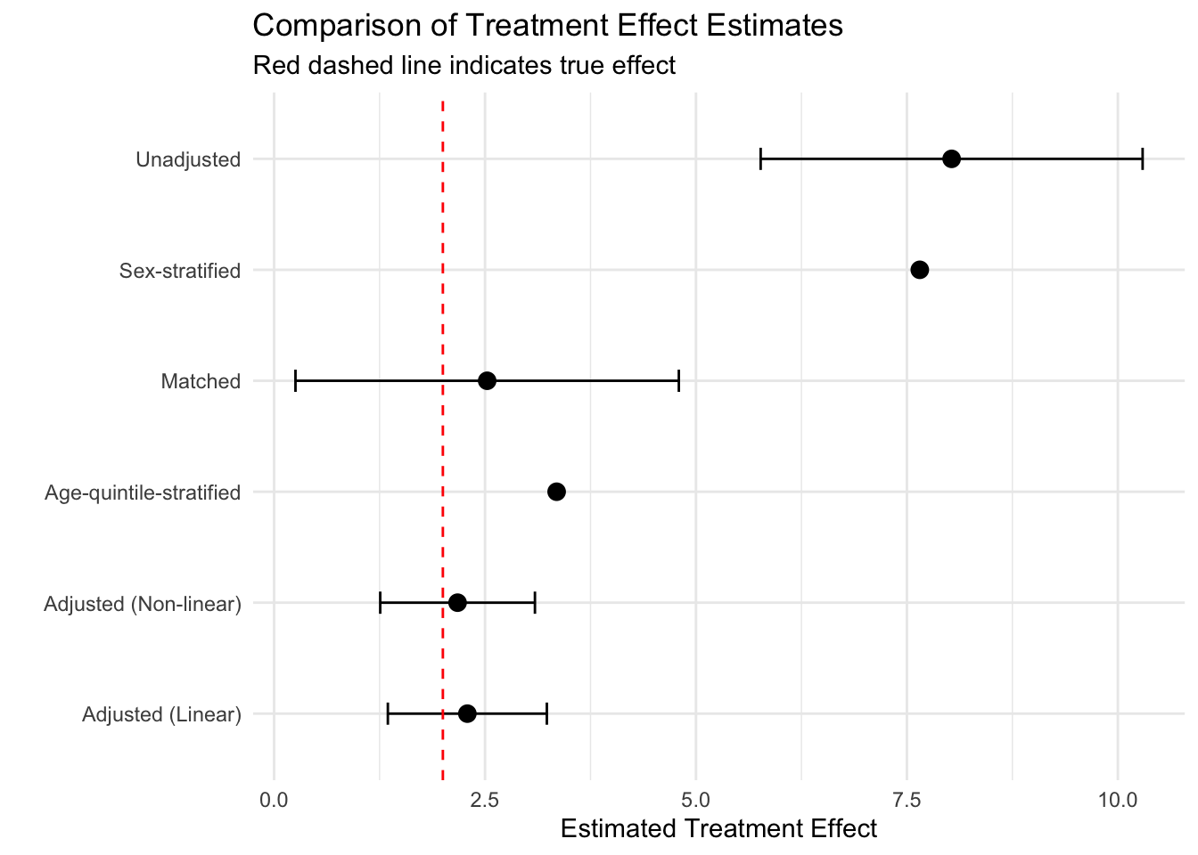
# 6. Visualization of different adjustment approaches
#-------------------------------------------------------------------------
# Prepare results for plotting
results <- data.frame(
  Method = c("Unadjusted", "Adjusted (Linear)", "Adjusted (Non-linear)", 
             "Sex-stratified", "Age-quintile-stratified", "Matched"),
  Estimate = c(coef(model_unadjusted)["treatmentB"],
               coef(model_adjusted)["treatmentB"],
               coef(model_nonlinear)["treatmentB"],
               avg_strat_effect_sex,
               avg_strat_effect_age,
               coef(matched_model)["treatmentB"]),
  SE = c(summary_unadjusted$coefficients["treatmentB", "Std. Error"],
         summary_adjusted$coefficients["treatmentB", "Std. Error"],
         summary_nonlinear$coefficients["treatmentB", "Std. Error"],
         NA,  # Would need bootstrap for proper SE
         NA,  # Would need bootstrap for proper SE
         summary_matched$coefficients["treatmentB", "Std. Error"])
)

results$Lower <- results$Estimate - 1.96 * results$SE
results$Upper <- results$Estimate + 1.96 * results$SE

# Plot the results
ggplot(results, aes(x = Method, y = Estimate)) +
  geom_point(size = 3) +
  geom_errorbar(aes(ymin = Lower, ymax = Upper), width = 0.2) +
  geom_hline(yintercept = true_effect, linetype = "dashed", color = "red") +
  labs(title = "Comparison of Treatment Effect Estimates",
       subtitle = "Red dashed line indicates true effect",
       y = "Estimated Treatment Effect",
       x = "") +
  theme_minimal() +
  coord_flip()

#-------------------------------------------------------------------------
# 7. Example from the n-table: checking BMI adequacy
#-------------------------------------------------------------------------
# Simulate height and weight data
n_bmi <- 300
log_height <- rnorm(n_bmi, mean = log(170), sd = 0.1)
log_weight <- -2 * log_height + rnorm(n_bmi, mean = log(70) + 2*log(170), sd = 0.2)

# Create some outcome related to BMI
bmi_outcome <- -2 * log_height + log_weight + rnorm(n_bmi, mean = 0, sd = 1)

# Check if coefficient ratio is approximately -2
bmi_model <- lm(bmi_outcome ~ log_height + log_weight)
summary_bmi <- summary(bmi_model)

cat("\nTesting if BMI adequately summarizes height and weight:\n")

Testing if BMI adequately summarizes height and weight:

cat("Log Height coefficient:", coef(bmi_model)["log_height"], "\n")

Log Height coefficient: -2.942465 

cat("Log Weight coefficient:", coef(bmi_model)["log_weight"], "\n")

Log Weight coefficient: 0.7942051 

cat("Ratio of coefficients (log_height/log_weight):", 
    coef(bmi_model)["log_height"]/coef(bmi_model)["log_weight"], "\n")

Ratio of coefficients (log_height/log_weight): -3.704918 

cat("If this ratio is close to -2, BMI adequately summarizes height and weight\n")

If this ratio is close to -2, BMI adequately summarizes height and weight

#-------------------------------------------------------------------------
# 8. Example: determining whether change or recent measurement is important
#-------------------------------------------------------------------------
# Simulate weights at two time points
n_weight <- 250
weight_1y_ago <- rnorm(n_weight, mean = 75, sd = 10)
weight_current <- weight_1y_ago + rnorm(n_weight, mean = -2, sd = 3) # slight weight loss on average

# Create outcome more strongly related to current weight
weight_outcome <- 0.1 * weight_1y_ago + 0.9 * weight_current + rnorm(n_weight, mean = 0, sd = 5)

# Fit model with both weights
weight_model <- lm(weight_outcome ~ weight_1y_ago + weight_current)
summary_weight <- summary(weight_model)

cat("\nDetermining importance of change vs. recent measurement:\n")

Determining importance of change vs. recent measurement:

cat("Weight 1y ago coefficient:", coef(weight_model)["weight_1y_ago"], "\n")

Weight 1y ago coefficient: 0.09458777 

cat("Current weight coefficient:", coef(weight_model)["weight_current"], "\n")

Current weight coefficient: 0.9164967 

cat("Ratio of coefficients (1y_ago/current):", 
    coef(weight_model)["weight_1y_ago"]/coef(weight_model)["weight_current"], "\n")

Ratio of coefficients (1y_ago/current): 0.1032058 

cat("If ratio is close to -1, change score is adequate\n")

If ratio is close to -1, change score is adequate

cat("If coefficient for weight 1y ago is very small, recent weight is most important\n")

If coefficient for weight 1y ago is very small, recent weight is most important

15.3