---
title: "TERN-701 CARDINAL Phase 1 Study Analysis"
subtitle: "Novel Allosteric BCR::ABL1 Inhibitor in Previously Treated CML"
author: "Clinical Analysis Report"
date: "`r Sys.Date()`"
format:
html:
toc: true
toc-depth: 3
toc-location: left
theme: journal
code-fold: true
code-tools: true
fig-width: 10
fig-height: 6
df-print: paged
execute:
warning: false
message: false
---
```{r setup}
#| include: false
# Load required libraries
library(tidyverse)
library(gt)
library(gtsummary)
library(patchwork)
library(plotly)
library(viridis)
library(scales)
library(kableExtra)
# Set theme
theme_set(theme_minimal(base_size = 12))
# Color palette for consistency
cml_colors <- c(
"TERN-701" = "#2E86AB",
"Response" = "#A23B72",
"Safety" = "#F18F01",
"Prior Treatment" = "#6C5B7B"
)
```
## Executive Summary
```{r summary-data}
# Create summary metrics
summary_metrics <- tibble(
  Metric = c("Enrolled Patients", "Median Age (years)", "Median Prior TKIs",
             "On Treatment", "MMR by 24 weeks", "Grade ≥3 TEAEs"),
  Value = c("55", "58 (29-86)", "3 (1-6)",
            "48 (87.3%)", "24/32 (75%)", "≤10% each"),
  Category = c("Enrollment", "Demographics", "Prior Treatment",
               "Retention", "Efficacy", "Safety")
)

summary_metrics %>%
  gt(groupname_col = "Category") %>%
  tab_header(
    title = "CARDINAL Study Key Metrics",
    subtitle = "Data cutoff: June 30, 2025"
  ) %>%
  cols_label(
    Metric = "Metric",
    Value = "Value"
  ) %>%
  tab_style(
    style = cell_fill(color = "#E8F4F8"),
    locations = cells_body(columns = everything(), rows = Category == "Efficacy")
  ) %>%
  tab_style(
    style = cell_text(weight = "bold"),
    locations = cells_body(columns = Metric)
  ) %>%
  tab_options(
    table.font.size = 14,
    heading.title.font.size = 16
  )
```
## Study Design
### Dose Escalation Cohorts
```{r dose-cohorts}
# Create dose escalation data
dose_data <- tibble(
  Cohort = 1:4,
  Dose = c(160, 320, 400, 500),
  `Dose Level` = paste0(Dose, " mg QD"),
  Status = c("Complete", "Complete", "Complete", "Complete"),
  RDE = c("No", "Yes", "No", "Yes")
)

dose_data %>%
  gt() %>%
  tab_header(title = "Part 1: Dose Escalation") %>%
  cols_label(
    Cohort = "Cohort",
    Dose = "Dose (mg)",
    `Dose Level` = "Dosing",
    Status = "Status",
    RDE = "Selected for Expansion"
  ) %>%
  tab_style(
    style = cell_fill(color = "#90EE90"),
    locations = cells_body(
      columns = everything(),
      rows = RDE == "Yes"
    )
  ) %>%
  tab_footnote(
    footnote = "RDE = Recommended Dose for Expansion",
    locations = cells_column_labels(columns = RDE)
  )
```
## Patient Characteristics
### Demographics and Baseline Disease
```{r patient-characteristics}
# Create patient characteristics data
patient_chars <- tibble(
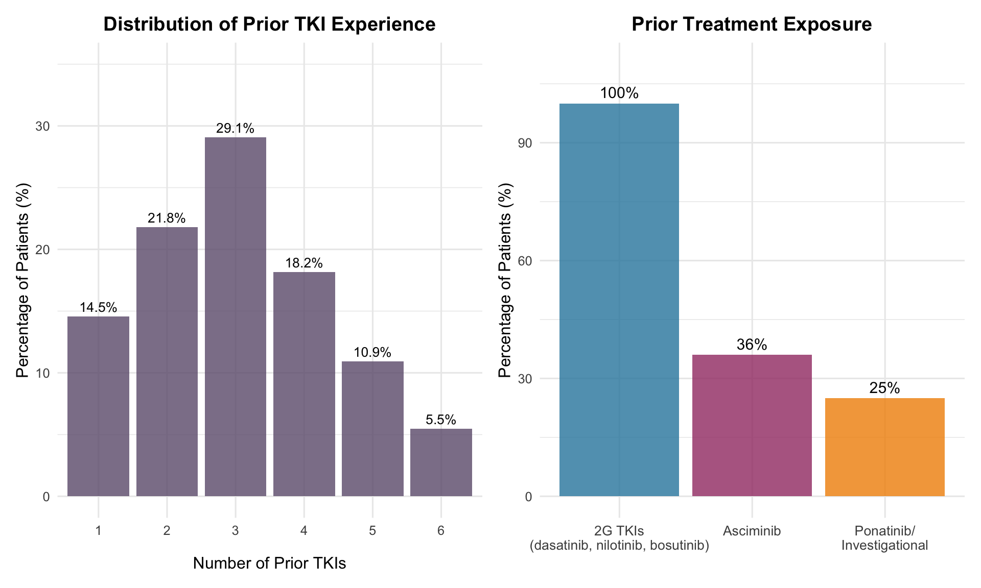
  Characteristic = c("Age, median (range)", "Male sex", "Prior TKIs, median (range)",
                    "≥4 prior TKIs", "Prior asciminib", "Prior ponatinib/investigational",
                    "Baseline BCR::ABL1 >1%", "Baseline BCR::ABL1 >10%",
                    "T315I mutation", "F317L mutation"),
  Value = c("58 (29-86)", "31 (56%)", "3 (1-6)", "19 (35%)", "20 (36%)",
           "14 (25%)", "31 (56%)", "24 (44%)", "5 (9%)", "2 (4%)"),
  N = 55
)

# Visualization of prior treatments
prior_tx_data <- tibble(
  `Prior TKIs` = c("1", "2", "3", "4", "5", "6"),
  Count = c(8, 12, 16, 10, 6, 3),  # Estimated from percentages
  Percentage = Count/55*100
)

p1 <- ggplot(prior_tx_data, aes(x = `Prior TKIs`, y = Percentage)) +
  geom_col(fill = cml_colors["Prior Treatment"], alpha = 0.8) +
  geom_text(aes(label = paste0(round(Percentage, 1), "%")),
            vjust = -0.5, size = 3.5) +
  labs(title = "Distribution of Prior TKI Experience",
       x = "Number of Prior TKIs",
       y = "Percentage of Patients (%)") +
  ylim(0, 35) +
  theme(plot.title = element_text(hjust = 0.5, face = "bold"))

# Prior specific TKIs
prior_specific <- tibble(
  Treatment = c("2G TKIs\n(dasatinib, nilotinib, bosutinib)",
                "Asciminib",
                "Ponatinib/\nInvestigational"),
  Percentage = c(100, 36, 25)
)

p2 <- ggplot(prior_specific, aes(x = reorder(Treatment, -Percentage),
                                  y = Percentage)) +
  geom_col(fill = c("#2E86AB", "#A23B72", "#F18F01"), alpha = 0.8) +
  geom_text(aes(label = paste0(Percentage, "%")),
            vjust = -0.5, size = 4) +
  labs(title = "Prior Treatment Exposure",
       x = "",
       y = "Percentage of Patients (%)") +
  ylim(0, 110) +
  theme(plot.title = element_text(hjust = 0.5, face = "bold"),
        axis.text.x = element_text(size = 10))

p1 + p2 + plot_layout(ncol = 2)
```
### Baseline BCR::ABL1 Levels
```{r bcr-abl-levels}
# Create BCR::ABL1 distribution data
bcr_abl_data <- tibble(
  Category = c("BCR::ABL1 ≤1%", "BCR::ABL1 1-10%", "BCR::ABL1 >10%"),
  Patients = c(24, 7, 24),  # Estimated from percentages
  Percentage = c(44, 12, 44)
)

# Create donut chart for BCR::ABL1 distribution
plot_ly(bcr_abl_data,
        labels = ~Category,
        values = ~Patients,
        text = ~paste(Patients, "patients\n(", Percentage, "%)", sep = ""),
        textposition = 'outside',
        textinfo = 'label+text',
        marker = list(colors = c("#E8F4F8", "#A8D8EA", "#2E86AB")),
        hole = 0.4) %>%
  add_pie() %>%
  layout(title = list(text = "<b>Baseline BCR::ABL1 Distribution</b>",
                     font = list(size = 16)),
         showlegend = FALSE,
         annotations = list(
           text = "N=55",
           x = 0.5,
           y = 0.5,
           xref = "paper",
           yref = "paper",
           showarrow = FALSE,
           font = list(size = 20)
         ))
```
## Efficacy Outcomes
### Major Molecular Response (MMR) by 24 Weeks
```{r efficacy-outcomes}
# Create efficacy data
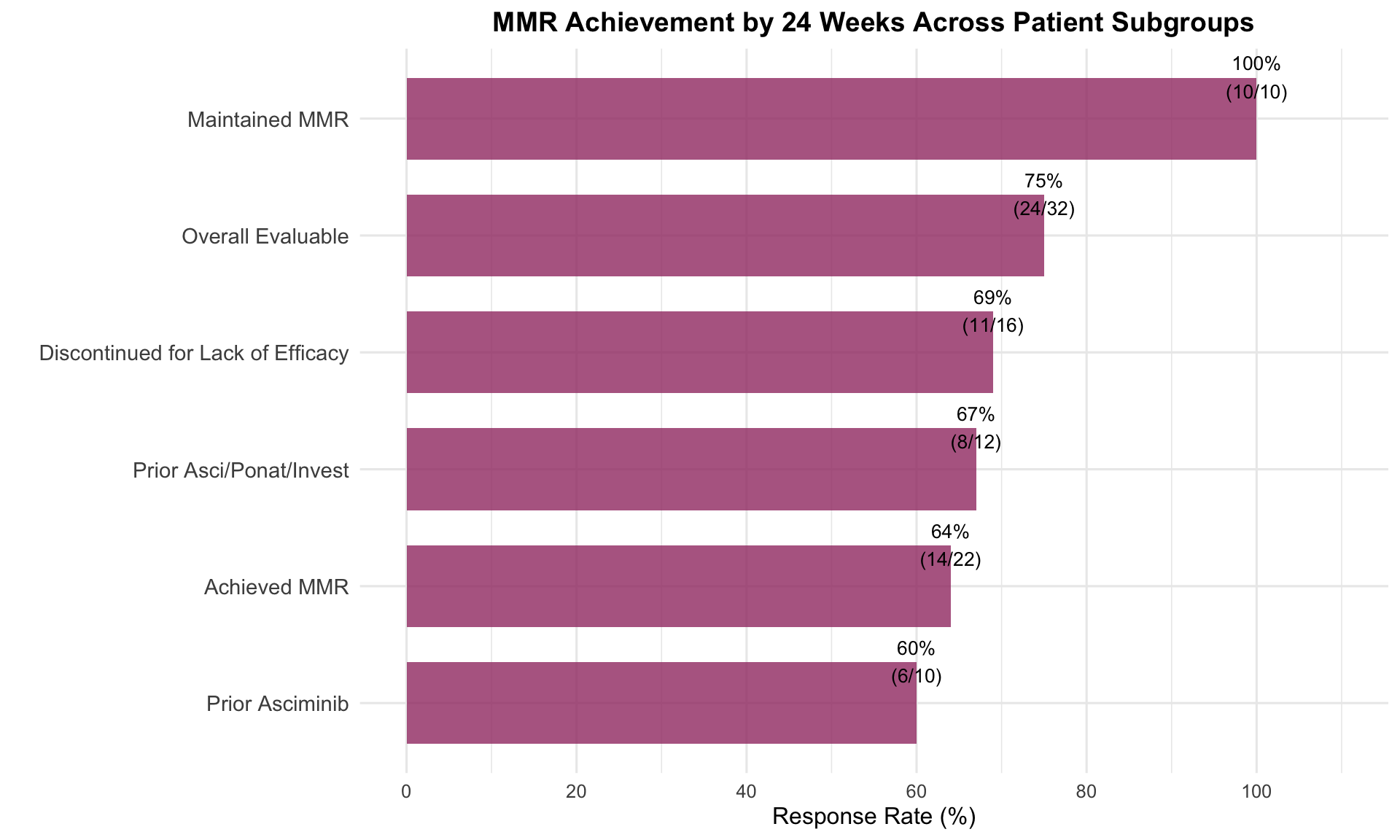
efficacy_data <- tibble(
  Population = c("Overall Evaluable", "Achieved MMR", "Maintained MMR",
                "Discontinued for Lack of Efficacy", "Prior Asciminib",
                "Prior Asci/Ponat/Invest"),
  `N Evaluable` = c(32, 22, 10, 16, 10, 12),
  `MMR by 24 weeks` = c(24, 14, 10, 11, 6, 8),
  `Response Rate` = c(75, 64, 100, 69, 60, 67)
)

# Create waterfall-style response plot
efficacy_plot_data <- efficacy_data %>%
  mutate(Population = factor(Population,
                             levels = Population[order(`Response Rate`)]))

ggplot(efficacy_plot_data, aes(x = Population, y = `Response Rate`)) +
  geom_col(fill = cml_colors["Response"], alpha = 0.8, width = 0.7) +
  geom_text(aes(label = paste0(`Response Rate`, "%\n(",
                               `MMR by 24 weeks`, "/", `N Evaluable`, ")")),
            vjust = -0.5, size = 3.5) +
  coord_flip() +
  labs(title = "MMR Achievement by 24 Weeks Across Patient Subgroups",
       x = "",
       y = "Response Rate (%)") +
  scale_y_continuous(limits = c(0, 110), breaks = seq(0, 100, 20)) +
  theme(plot.title = element_text(hjust = 0.5, face = "bold", size = 14),
        axis.text.y = element_text(size = 11))
```
### Response Dynamics
```{r response-dynamics}
# Create response tracking table
response_tracking <- tibble(
  `Response Metric` = c("Achieved MMR (no baseline MMR)",
                       "Maintained MMR (baseline MMR)",
                       "Lost MMR at data cutoff"),
  `n/N` = c("14/22", "10/10", "0/24"),
  `Rate (%)` = c(64, 100, 0),
  `Interpretation` = c("Strong de novo response",
                       "Excellent maintenance",
                       "Durable responses")
)

response_tracking %>%
  gt() %>%
  tab_header(
    title = "Response Dynamics Analysis",
    subtitle = "Key efficacy endpoints"
  ) %>%
  cols_label(
    `Response Metric` = "Metric",
    `n/N` = "n/N",
    `Rate (%)` = "Rate (%)",
    Interpretation = "Clinical Interpretation"
  ) %>%
  tab_style(
    style = list(
      cell_fill(color = "#90EE90"),
      cell_text(weight = "bold")
    ),
    locations = cells_body(
      columns = everything(),
      rows = `Rate (%)` == 100
    )
  )
```
## Safety Profile
### Treatment-Emergent Adverse Events (TEAEs)
```{r safety-profile}
# Create safety data
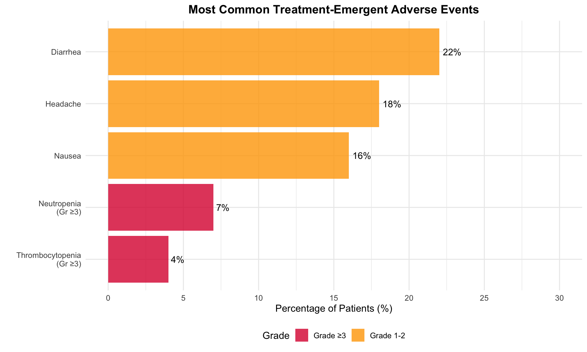
safety_data <- tibble(
  `Adverse Event` = c("Any TEAE", "Diarrhea", "Headache", "Nausea",
                     "Neutropenia (Grade ≥3)", "Thrombocytopenia (Grade ≥3)"),
  `All Grades n (%)` = c("41 (74)", "12 (22)", "10 (18)", "9 (16)",
                        "4 (7)", "2 (4)"),
  `Grade ≥3 n (%)` = c("NA", "0", "0", "0", "4 (7)", "2 (4)"),
  Category = c("Overall", "GI", "Neurological", "GI",
              "Hematologic", "Hematologic")
)

# Visualization of common AEs
ae_plot_data <- tibble(
  AE = c("Diarrhea", "Headache", "Nausea", "Neutropenia\n(Gr ≥3)",
         "Thrombocytopenia\n(Gr ≥3)"),
  Percentage = c(22, 18, 16, 7, 4),
  Grade = c("Grade 1-2", "Grade 1-2", "Grade 1-2", "Grade ≥3", "Grade ≥3")
)

ggplot(ae_plot_data, aes(x = reorder(AE, Percentage), y = Percentage, fill = Grade)) +
  geom_col(alpha = 0.8) +
  geom_text(aes(label = paste0(Percentage, "%")), hjust = -0.2, size = 4) +
  coord_flip() +
  scale_fill_manual(values = c("Grade 1-2" = "#FFA500", "Grade ≥3" = "#DC143C")) +
  labs(title = "Most Common Treatment-Emergent Adverse Events",
       x = "",
       y = "Percentage of Patients (%)") +
  scale_y_continuous(limits = c(0, 30), breaks = seq(0, 30, 5)) +
  theme(plot.title = element_text(hjust = 0.5, face = "bold"),
        legend.position = "bottom")
```
### Treatment Discontinuations
```{r discontinuations}
# Create discontinuation data
discontinuation_data <- tibble(
  Reason = c("Disease Progression", "Adverse Events",
             "Consent Withdrawal/Lost to Follow-up"),
  Count = c(4, 1, 2),
  Percentage = round(Count/55*100, 1)
)

# Create pie chart for discontinuations
plot_ly(discontinuation_data,
        labels = ~Reason,
        values = ~Count,
        text = ~paste(Count, "patients\n(", Percentage, "%)", sep = ""),
        textposition = 'outside',
        textinfo = 'text',
        marker = list(colors = c("#DC143C", "#FFA500", "#808080"))) %>%
  add_pie() %>%
  layout(title = list(text = "<b>Reasons for Treatment Discontinuation (n=7)</b>",
                     font = list(size = 14)),
         showlegend = TRUE,
         legend = list(x = 0.85, y = 0.5))
```
## Comparative Context
### TERN-701 vs Historical Allosteric Inhibitor Data
```{r comparative-analysis}
# Create comparative table (hypothetical comparison with asciminib)
comparative_data <- tibble(
  Parameter = c("Dose Range Tested", "RDE Selected", "Prior Asciminib Allowed",
               "MMR by 24 weeks (overall)", "MMR in asciminib-exposed",
               "Grade ≥3 Neutropenia", "Grade ≥3 Thrombocytopenia"),
  `TERN-701\n(CARDINAL)` = c("160-500 mg QD", "320, 500 mg QD", "Yes (36%)",
                             "75% (24/32)", "60% (6/10)", "7%", "4%"),
  `Historical Context` = c("Variable", "Variable", "No/Limited",
                          "Variable", "Limited data", "Variable", "Variable")
)

comparative_data %>%
  gt() %>%
  tab_header(
    title = "TERN-701 Positioning in Allosteric Inhibitor Landscape",
    subtitle = "Key differentiating features"
  ) %>%
  cols_label(
    Parameter = "",
    `TERN-701\n(CARDINAL)` = "TERN-701 (CARDINAL)",
    `Historical Context` = "Historical Context"
  ) %>%
  tab_style(
    style = cell_fill(color = "#E8F4F8"),
    locations = cells_body(
      columns = `TERN-701\n(CARDINAL)`,
      rows = grepl("MMR|asciminib", Parameter)
    )
  ) %>%
  tab_style(
    style = cell_text(weight = "bold"),
    locations = cells_body(columns = Parameter)
  )
```
## Key Takeaways
```{r key-takeaways}
takeaways <- tibble(
  Category = c("Efficacy", "Efficacy", "Safety", "Safety", "Population", "Next Steps"),
  Finding = c(
    "75% MMR rate by 24 weeks in heavily pretreated population",
    "Activity maintained in asciminib-exposed patients (60% MMR)",
    "Favorable tolerability with 74% of TEAEs being low grade",
    "No DLTs observed, MTD not reached up to 500 mg QD",
    "Median 3 prior TKIs with 36% having prior asciminib exposure",
    "320 mg and 500 mg QD selected as RDEs for randomized expansion"
  ),
  Significance = c(
    "High",
    "High",
    "Moderate",
    "Moderate",
    "High",
    "High"
  )
)

takeaways %>%
  gt(groupname_col = "Category") %>%
  tab_header(
    title = "Clinical Significance Summary"
  ) %>%
  cols_label(
    Finding = "Key Finding",
    Significance = "Clinical Impact"
  ) %>%
  tab_style(
    style = cell_text(weight = "bold", color = "#2E86AB"),
    locations = cells_body(
      columns = Significance,
      rows = Significance == "High"
    )
  ) %>%
  tab_style(
    style = cell_fill(color = "#F0F8FF"),
    locations = cells_row_groups()
  )
```
## Conclusions
::: callout-note
## Study Implications
TERN-701 demonstrates promising efficacy and safety in a heavily pretreated CML-CP population, including patients with prior exposure to asciminib and other investigational TKIs. The 75% MMR rate by 24 weeks, combined with favorable tolerability profile, supports continued development in the randomized dose expansion phase.
:::
::: callout-important
## Data Limitations
- Phase 1 dose-escalation design with limited sample size (N=55)
- Median follow-up of 4.5 months requires longer-term assessment
- Cross-trial comparisons should be interpreted with caution
- Full safety profile will emerge with expanded enrollment
:::
```{r session-info}
#| echo: false
#| eval: false
sessionInfo()
```
------------------------------------------------------------------------