2 FDA Guidance on Bayesian Methodology in Clinical Trials
2.1 FDA Draft Guidance on Bayesian Methodology (January 2026)
“Use of Bayesian Methodology in Clinical Trials of Drug and Biological Products”
With critical appraisal from Stephen Senn’s “Beware of the Morlocks” (March 2026) and Frank Harrell’s Statistical Thinking framework
Prepared for Blood Cancer Talks podcast episode
3 Executive Summary
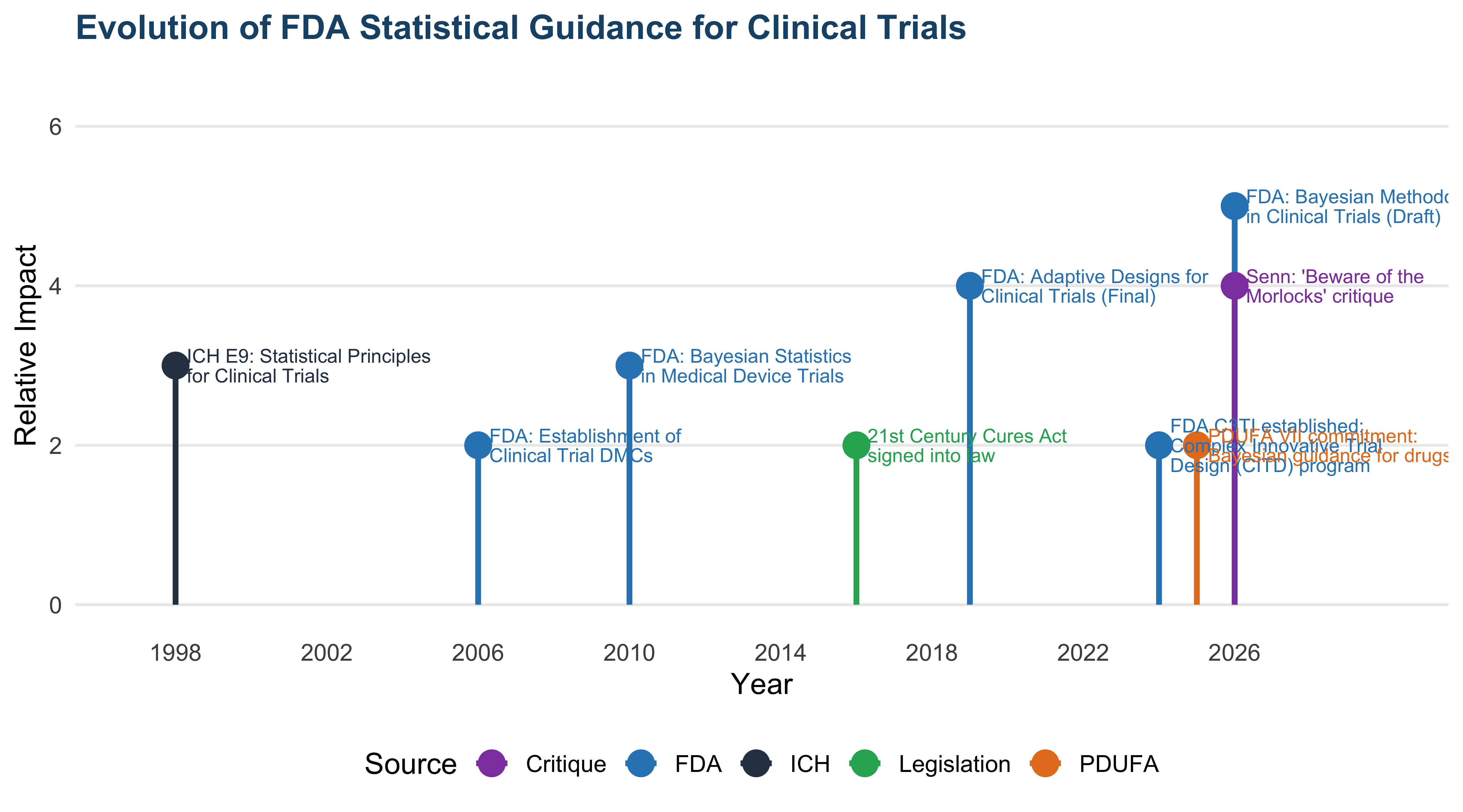
On January 12, 2026, the FDA released a landmark draft guidance on the use of Bayesian methodology in clinical trials, building upon the November 2019 Adaptive Designs Guidance. This document signals a formal regulatory shift toward accepting Bayesian primary inference in pivotal confirmatory trials.
The draft guidance is open for comment until March 13, 2026 (Docket No. FDA-2025-D-3217). Comments may be submitted via regulations.gov.
This companion document provides:
- A comprehensive summary of both FDA guidances (2019 Adaptive Designs & 2026 Bayesian)
- R and Python visualizations illustrating key statistical concepts
- Stephen Senn’s critique of the Bayesian Time Machine and platform trial designs
- Frank Harrell’s perspectives on Bayesian clinical trial methodology
- Practical implications for hematology-oncology trial design
4 Historical Context and Regulatory Timeline
Show code
library(ggplot2)

timeline <- data.frame(
  year = c(1998, 2006, 2010, 2016, 2019, 2024, 2025, 2026, 2026),
  event = c(
    "ICH E9: Statistical Principles\nfor Clinical Trials",
    "FDA: Establishment of\nClinical Trial DMCs",
    "FDA: Bayesian Statistics\nin Medical Device Trials",
    "21st Century Cures Act\nsigned into law",
    "FDA: Adaptive Designs for\nClinical Trials (Final)",
    "FDA C3TI established;\nComplex Innovative Trial\nDesign (CITD) program",
    "PDUFA VII commitment:\nBayesian guidance for drugs",
    "FDA: Bayesian Methodology\nin Clinical Trials (Draft)",
    "Senn: 'Beware of the\nMorlocks' critique"
  ),
  category = c("ICH", "FDA", "FDA", "Legislation", "FDA", "FDA", "PDUFA", "FDA", "Critique"),
  importance = c(3, 2, 3, 2, 4, 2, 2, 5, 4)
)

pal <- c("ICH" = "#2c3e50", "FDA" = "#2e86c1", "Legislation" = "#27ae60",
          "PDUFA" = "#e67e22", "Critique" = "#8e44ad")

ggplot(timeline, aes(x = year, y = importance, color = category)) +
  geom_segment(aes(xend = year, y = 0, yend = importance), linewidth = 1.2) +
  geom_point(size = 5) +
  geom_text(aes(label = event), hjust = 0, nudge_x = 0.3, size = 3,
            lineheight = 0.85, fontface = "plain", show.legend = FALSE) +
  scale_color_manual(values = pal, name = "Source") +
  scale_x_continuous(breaks = seq(1998, 2026, 4), limits = c(1997, 2030)) +
  scale_y_continuous(limits = c(0, 6.5)) +
  labs(x = "Year", y = "Relative Impact",
       title = "Evolution of FDA Statistical Guidance for Clinical Trials") +
  theme_minimal(base_size = 13) +
  theme(
    plot.title = element_text(face = "bold", color = "#1a5276", size = 15),
    panel.grid.minor = element_blank(),
    panel.grid.major.x = element_blank(),
    legend.position = "bottom"
  )
5 Frequentist vs. Bayesian Inference
5.0.0.1 Frequentist Framework
Question answered: If the drug has no effect, how likely is data this extreme?
- p-value = P(data ≥ observed | H₀ true)
- Conditions on the unknown (H₀), computes probability of known (data)
- Depends on what might have happened (sample space)
- Requires complex adjustments for multiple looks
- Type I error rate α = long-run false positive rate
5.0.0.2 Bayesian Framework
Question answered: Given the data, what is the probability the drug works?
- Posterior = P(θ | data, prior)
- Conditions on the known (data), computes probability of unknown (θ)
- Depends only on what did happen
- No multiplicity adjustments needed for sequential looks
- Posterior probability = direct probability of efficacy
Show code
import numpy as np
import matplotlib.pyplot as plt
from matplotlib.patches import FancyBboxPatch
import matplotlib.patches as mpatches

fig, axes = plt.subplots(1, 2, figsize=(12, 5))

# ---- Panel A: Frequentist p-value as function of sample size & effect ----
ax = axes[0]
n_values = np.arange(20, 501, 5)
effect_sizes = [0.2, 0.35, 0.5]
colors_freq = ['#e74c3c', '#e67e22', '#c0392b']

for es, col in zip(effect_sizes, colors_freq):
    se = 1.0 / np.sqrt(n_values)
    z = es / se
    from scipy import stats
    pvals = 1 - stats.norm.cdf(z)
    ax.plot(n_values, pvals, color=col, linewidth=2.2, label=f'δ = {es}')

ax.axhline(y=0.025, color='grey', linestyle='--', linewidth=1, alpha=0.7)
ax.text(480, 0.032, 'α = 0.025', fontsize=9, color='grey', ha='right')
ax.set_xlabel('Sample Size (per arm)', fontsize=12)
ax.set_ylabel('One-sided p-value', fontsize=12)
ax.set_title('Frequentist: p-value Depends on\nSample Size & Effect', fontsize=13, fontweight='bold', color='#c0392b')
ax.set_ylim(-0.01, 0.35)
(-0.01, 0.35)Show code
ax.legend(title='True effect (δ)', fontsize=10)
ax.spines['top'].set_visible(False)
ax.spines['right'].set_visible(False)

# ---- Panel B: Bayesian posterior probability ----
ax2 = axes[1]
# Simulate posterior P(δ > 0) for skeptical prior
prior_mean = 0.0
prior_sd_values = [0.5, 1.0, 2.0]  # skeptical to diffuse
observed_effect = np.linspace(-0.2, 0.8, 200)
n = 200
se_obs = 1.0 / np.sqrt(n)

colors_bayes = ['#1abc9c', '#27ae60', '#2ecc71']
labels = ['Skeptical (σ₀=0.5)', 'Moderate (σ₀=1.0)', 'Diffuse (σ₀=2.0)']

for prior_sd, col, lab in zip(prior_sd_values, colors_bayes, labels):
    post_mean = (prior_mean / prior_sd**2 + observed_effect / se_obs**2) / (1/prior_sd**2 + 1/se_obs**2)
    post_var = 1 / (1/prior_sd**2 + 1/se_obs**2)
    post_sd = np.sqrt(post_var)
    prob_eff = 1 - stats.norm.cdf(0, loc=post_mean, scale=post_sd)
    ax2.plot(observed_effect, prob_eff, color=col, linewidth=2.2, label=lab)

ax2.axhline(y=0.975, color='grey', linestyle='--', linewidth=1, alpha=0.7)
ax2.text(0.78, 0.955, 'P(δ>0) = 0.975', fontsize=9, color='grey', ha='right')
ax2.axhline(y=0.95, color='grey', linestyle=':', linewidth=1, alpha=0.5)
ax2.set_xlabel('Observed Treatment Effect (δ̂)', fontsize=12)
ax2.set_ylabel('P(δ > 0 | data, prior)', fontsize=12)
ax2.set_title('Bayesian: Posterior Probability\nIncorporates Prior Belief', fontsize=13, fontweight='bold', color='#1a6e4e')
ax2.set_ylim(-0.02, 1.05)
(-0.02, 1.05)Show code
ax2.legend(title='Prior specification', fontsize=10)
ax2.spines['top'].set_visible(False)
ax2.spines['right'].set_visible(False)

plt.tight_layout()
plt.savefig('freq_vs_bayes.png', dpi=300, bbox_inches='tight')
plt.show()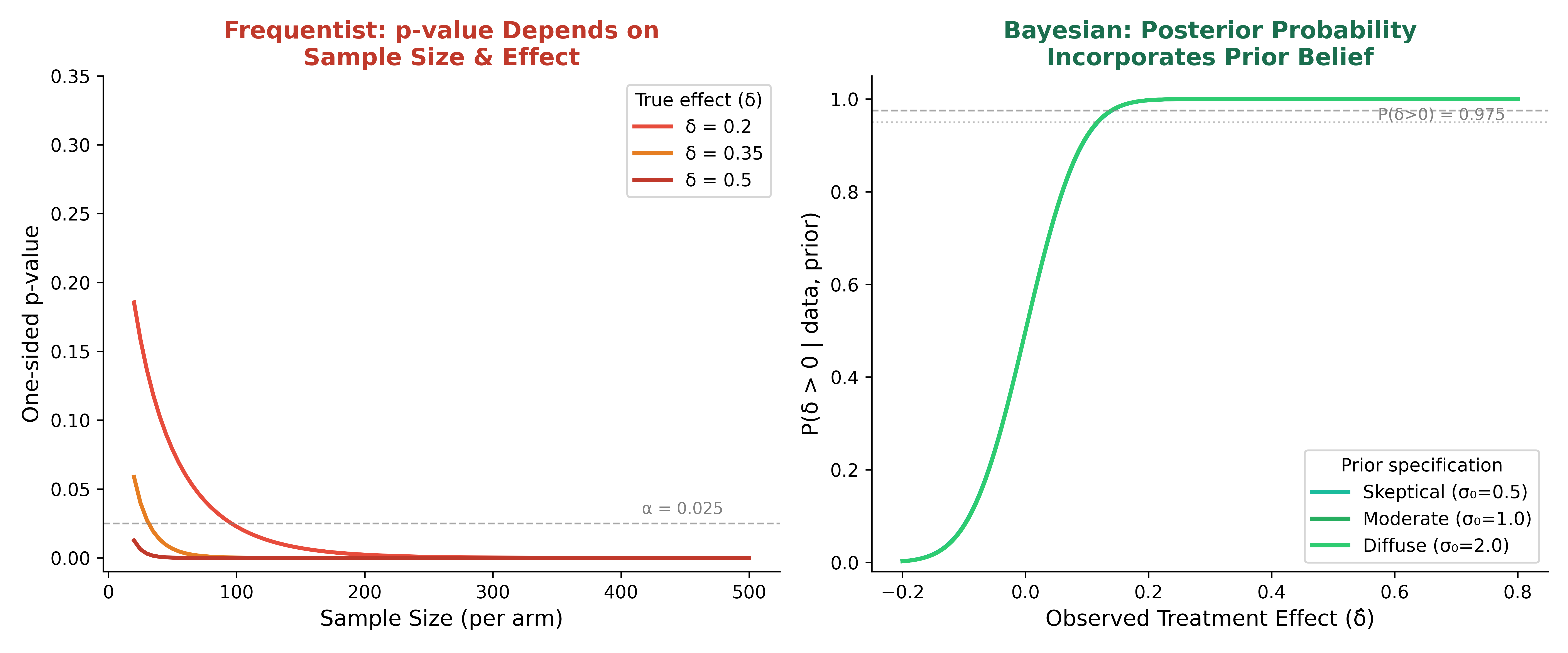
“Mixing a Bayesian probability that an assertion is true and a frequentist probability of making an assertion if you magically knew the treatment to be ignorable is like mixing apples and coconuts, and the frequentist nut is hard to crack.” ::: {.attribution} — Frank Harrell, Statistical Thinking (2023)
:::
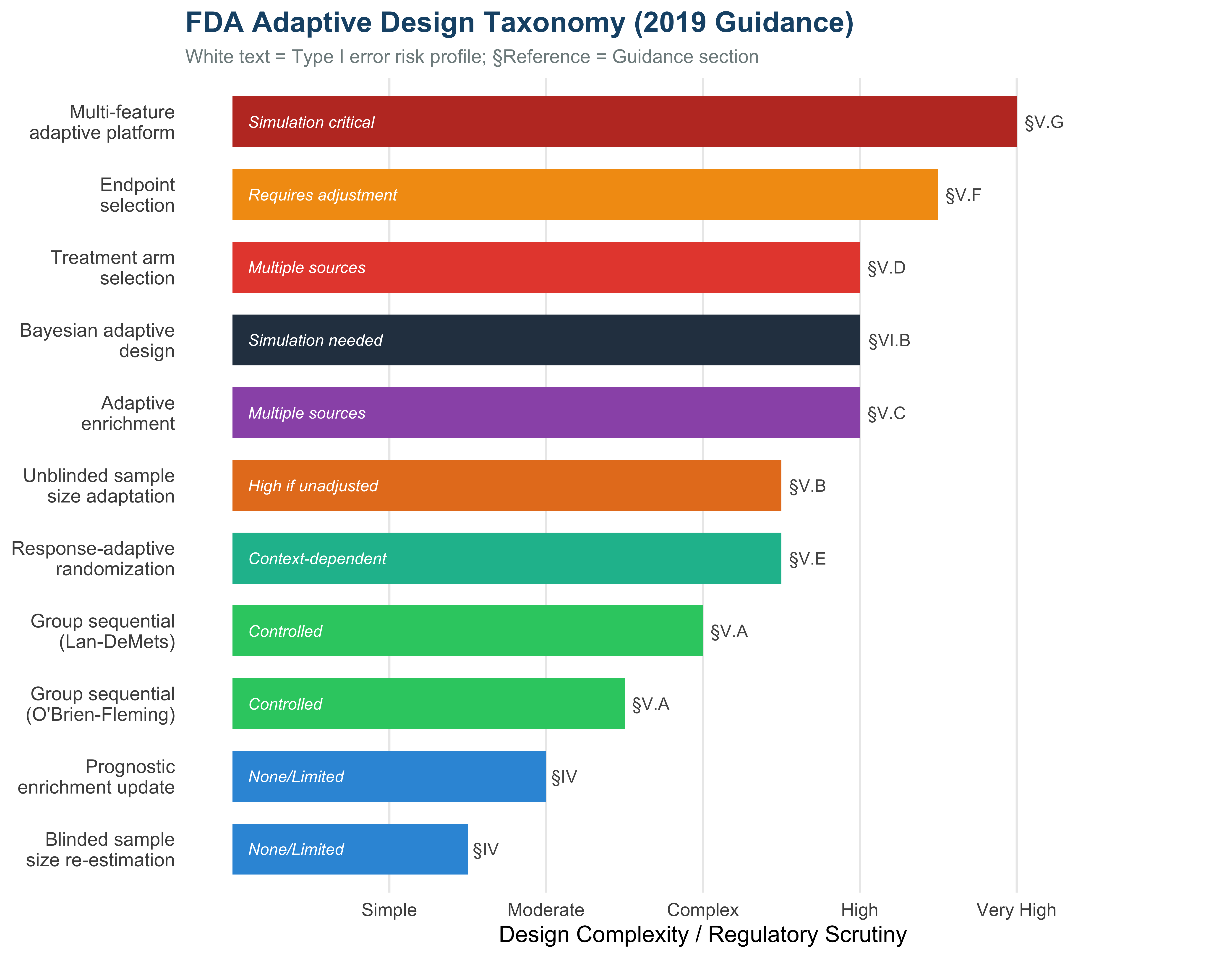
6 The 2019 FDA Adaptive Designs Guidance
The November 2019 guidance defines an adaptive design as:
A clinical trial design that allows for prospectively planned modifications to one or more aspects of the design based on accumulating data from subjects in the trial.
6.1 Taxonomy of Adaptive Designs
Show code
library(ggplot2)

designs <- data.frame(
  design = c(
    "Blinded sample\nsize re-estimation",
    "Prognostic\nenrichment update",
    "Group sequential\n(O'Brien-Fleming)",
    "Group sequential\n(Lan-DeMets)",
    "Unblinded sample\nsize adaptation",
    "Adaptive\nenrichment",
    "Treatment arm\nselection",
    "Response-adaptive\nrandomization",
    "Endpoint\nselection",
    "Bayesian adaptive\ndesign",
    "Multi-feature\nadaptive platform"
  ),
  data_type = c(
    "Non-comparative", "Non-comparative",
    "Comparative", "Comparative", "Comparative",
    "Comparative", "Comparative", "Comparative",
    "Comparative", "Either", "Both"
  ),
  complexity = c(1.5, 2, 2.5, 3, 3.5, 4, 4, 3.5, 4.5, 4, 5),
  type1_risk = c(
    "None/Limited", "None/Limited",
    "Controlled", "Controlled", "High if unadjusted",
    "Multiple sources", "Multiple sources", "Context-dependent",
    "Requires adjustment", "Simulation needed", "Simulation critical"
  ),
  section = c("IV", "IV", "V.A", "V.A", "V.B", "V.C", "V.D", "V.E", "V.F", "VI.B", "V.G"),
  color_group = c("non-comp", "non-comp", "gsd", "gsd", "sample",
                   "enrichment", "arm-select", "rar", "endpoint", "bayesian", "platform")
)

pal <- c("non-comp" = "#3498db", "gsd" = "#2ecc71", "sample" = "#e67e22",
         "enrichment" = "#9b59b6", "arm-select" = "#e74c3c", "rar" = "#1abc9c",
         "endpoint" = "#f39c12", "bayesian" = "#2c3e50", "platform" = "#c0392b")

ggplot(designs, aes(x = complexity, y = reorder(design, complexity), fill = color_group)) +
  geom_col(width = 0.7, show.legend = FALSE) +
  geom_text(aes(label = paste0("§", section)), hjust = -0.2, size = 3.2, color = "#555") +
  geom_text(aes(label = type1_risk, x = 0.1), hjust = 0, size = 3, color = "white", fontface = "italic") +
  scale_fill_manual(values = pal) +
  scale_x_continuous(limits = c(0, 6), breaks = 1:5,
                     labels = c("Simple", "Moderate", "Complex", "High", "Very High")) +
  labs(x = "Design Complexity / Regulatory Scrutiny", y = NULL,
       title = "FDA Adaptive Design Taxonomy (2019 Guidance)",
       subtitle = "White text = Type I error risk profile; §Reference = Guidance section") +
  theme_minimal(base_size = 12) +
  theme(
    plot.title = element_text(face = "bold", color = "#1a5276", size = 15),
    plot.subtitle = element_text(color = "#7f8c8d", size = 10),
    panel.grid.major.y = element_blank(),
    panel.grid.minor = element_blank(),
    axis.text.y = element_text(size = 10)
  )
6.2 Four Key Principles
The 2019 guidance establishes four principles for adaptive designs intended to provide substantial evidence of effectiveness:
Controlling the Chance of Erroneous Conclusions
Multiple adaptive features can inflate Type I error probability in subtle ways:
- Group sequential designs: Multiple hypothesis tests at interim analyses
- Adaptive enrichment: Population selection + multiple population testing
- Sample size re-estimation: Indiscriminate modification can more than double the Type I error rate
The guidance recommends simulation-based evaluation when analytical methods are unavailable, with 100,000 iterations per scenario for precise Type I error estimation (95% CI width ≈ ±0.1%).
Estimating Treatment Effects Reliably
Adaptive features can introduce systematic bias in treatment effect estimates:
- Early stopping for efficacy → overestimation of true effect
- Adaptive enrichment → biased subgroup estimates
- Confidence intervals may not have correct coverage probabilities
Methods exist for some designs (Jennison & Turnbull 1999) but are rarely applied in practice — a point Frank Harrell has emphasized.
Complete Prospective Planning
All adaptive features must be prespecified:
- Number and timing of interim analyses
- Specific adaptation algorithms
- Statistical inferential methods
- Success/futility criteria
This prevents post-hoc modifications motivated by unplanned knowledge of accumulating data.
Maintaining Trial Conduct
Access to comparative interim results must be limited to independent individuals. Knowledge of accumulating data can adversely affect:
- Patient accrual and retention
- Treatment adherence
- Endpoint assessment
- Investigator behavior
6.3 Group Sequential Designs: The α-Spending Problem
Show code
library(ggplot2)

# Approximate O'Brien-Fleming and Pocock boundaries for 4 equally-spaced looks
info_frac <- c(0.25, 0.50, 0.75, 1.00)

# O'Brien-Fleming z-boundaries (approximate)
obf_z <- c(4.05, 2.86, 2.34, 2.02)
# Pocock z-boundaries (approximate)
poc_z <- c(2.36, 2.36, 2.36, 2.36)
# Nominal (unadjusted) boundary
nom_z <- rep(qnorm(0.975), 4)

# Convert to one-sided p-values
obf_p <- 1 - pnorm(obf_z)
poc_p <- 1 - pnorm(poc_z)
nom_p <- rep(0.025, 4)

# Cumulative alpha spent
obf_alpha_cum <- c(0.00003, 0.0020, 0.0094, 0.0250)
poc_alpha_cum <- c(0.0091, 0.0164, 0.0218, 0.0250)

df_boundaries <- data.frame(
  look = rep(1:4, 3),
  info = rep(info_frac, 3),
  z_boundary = c(obf_z, poc_z, nom_z),
  method = rep(c("O'Brien-Fleming", "Pocock", "Nominal (no adjustment)"), each = 4)
)

df_alpha <- data.frame(
  look = rep(1:4, 2),
  info = rep(info_frac, 2),
  alpha_cum = c(obf_alpha_cum, poc_alpha_cum),
  method = rep(c("O'Brien-Fleming", "Pocock"), each = 4)
)

pal <- c("O'Brien-Fleming" = "#2e86c1", "Pocock" = "#e67e22", "Nominal (no adjustment)" = "#bdc3c7")

p1 <- ggplot(df_boundaries, aes(x = info, y = z_boundary, color = method)) +
  geom_line(linewidth = 1.3) +
  geom_point(size = 3.5) +
  scale_color_manual(values = pal) +
  labs(x = "Information Fraction", y = "Z-boundary (critical value)",
       title = "Stopping Boundaries for Efficacy",
       color = "Method") +
  theme_minimal(base_size = 12) +
  theme(plot.title = element_text(face = "bold", color = "#1a5276"),
        legend.position = "bottom")

p2 <- ggplot(df_alpha, aes(x = info, y = alpha_cum, color = method, fill = method)) +
  geom_area(alpha = 0.15, position = "identity") +
  geom_line(linewidth = 1.3) +
  geom_point(size = 3.5) +
  geom_hline(yintercept = 0.025, linetype = "dashed", color = "grey40") +
  annotate("text", x = 0.15, y = 0.027, label = "α = 0.025", size = 3.5, color = "grey40") +
  scale_color_manual(values = pal[1:2]) +
  scale_fill_manual(values = pal[1:2]) +
  labs(x = "Information Fraction", y = "Cumulative α spent",
       title = "Alpha-Spending Functions",
       color = "Method", fill = "Method") +
  theme_minimal(base_size = 12) +
  theme(plot.title = element_text(face = "bold", color = "#1a5276"),
        legend.position = "bottom")

library(patchwork)
p1 + p2 + plot_layout(guides = "collect") & theme(legend.position = "bottom")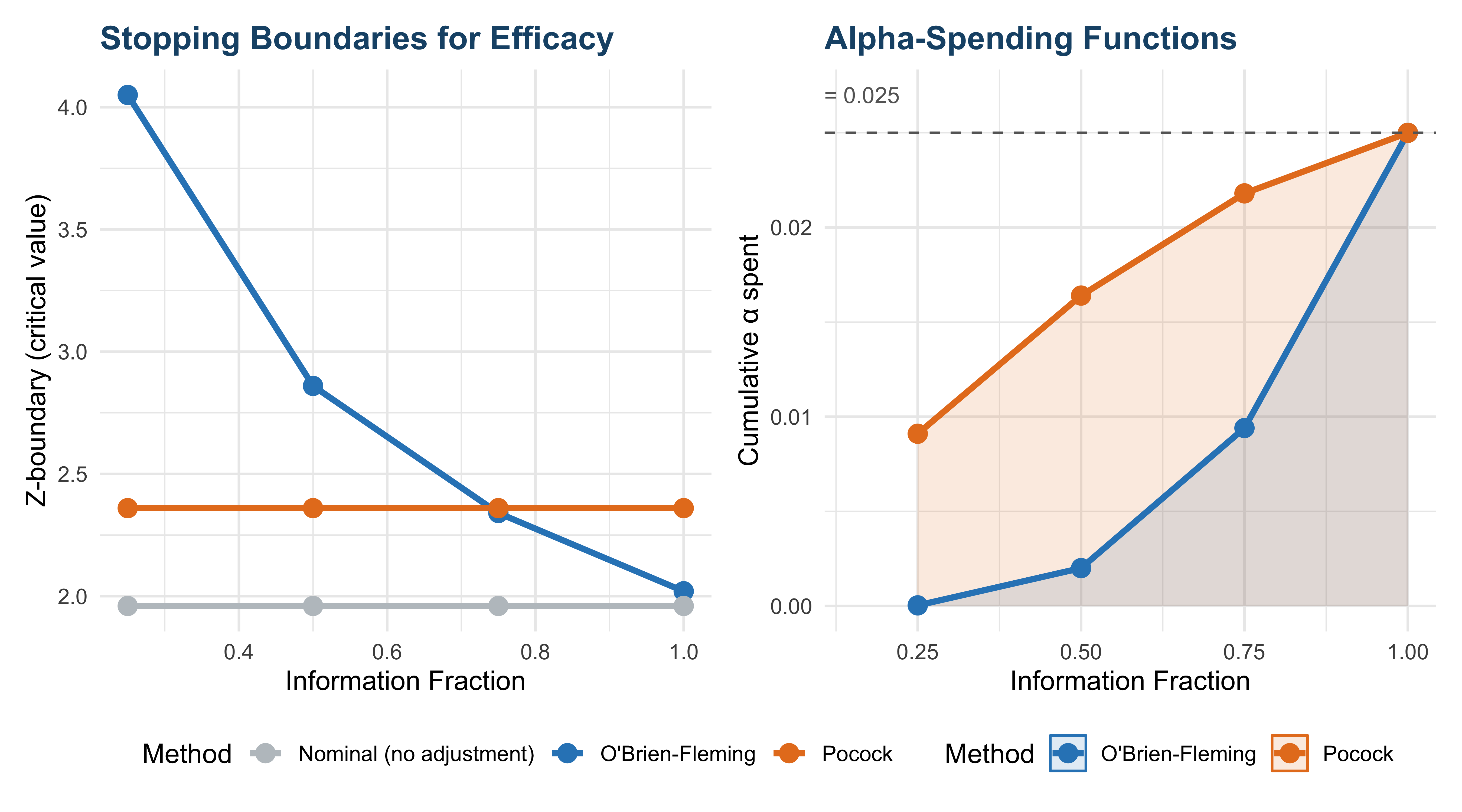
Frank Harrell argues that α-spending is fundamentally illogical from a Bayesian perspective. In his severe asthma trial case study, a planned interim analysis that never occurred still penalized the final analysis through the α-spending framework. He writes: “α considers intentions to analyze. α has nothing to do with the chance of making a decision error.”
7 The 2026 Bayesian Guidance: Core Framework
7.1 Three Pillars of the Guidance
Show code
import matplotlib.pyplot as plt
import matplotlib.patches as mpatches
import numpy as np

fig, ax = plt.subplots(1, 1, figsize=(11, 6))
ax.set_xlim(0, 12)
(0.0, 12.0)Show code
ax.set_ylim(0, 8)(0.0, 8.0)Show code
ax.axis('off')(np.float64(0.0), np.float64(12.0), np.float64(0.0), np.float64(8.0))Show code
# Title
ax.text(6, 7.5, 'FDA 2026 Bayesian Guidance: Three Core Pillars',
        fontsize=16, fontweight='bold', ha='center', color='#1a5276')

pillars = [
    {
        'x': 1.5, 'color': '#2e86c1',
        'title': 'Success Criteria',
        'items': [
            'Posterior probability\nP(θ > θ₀ | data) > c',
            'Benefit-risk &\ndecision-theoretic\napproaches',
            'Not limited to\nType I error calibration'
        ]
    },
    {
        'x': 5.0, 'color': '#27ae60',
        'title': 'Prior Specification',
        'items': [
            'Principled prior\nconstruction',
            'Sensitivity analyses\n(stress-testing)',
            'Safeguards for\nborrowing external\ninformation'
        ]
    },
    {
        'x': 8.5, 'color': '#8e44ad',
        'title': 'Operating\nCharacteristics',
        'items': [
            'Prospective evaluation\nvia simulation',
            'Bayesian power /\nassurance metrics',
            'Document computational\nmethods & convergence'
        ]
    }
]

for p in pillars:
    # Pillar rectangle
    rect = mpatches.FancyBboxPatch((p['x'] - 1.2, 0.3), 2.8, 6.2,
                                     boxstyle="round,pad=0.15",
                                     facecolor=p['color'], alpha=0.1,
                                     edgecolor=p['color'], linewidth=2.5)
    ax.add_patch(rect)

    # Pillar top
    top_rect = mpatches.FancyBboxPatch((p['x'] - 1.1, 5.2), 2.6, 1.1,
                                        boxstyle="round,pad=0.1",
                                        facecolor=p['color'], alpha=0.85,
                                        edgecolor='none')
    ax.add_patch(top_rect)
    ax.text(p['x'] + 0.2, 5.75, p['title'], fontsize=11, fontweight='bold',
            color='white', ha='center', va='center')

    for i, item in enumerate(p['items']):
        y_pos = 4.3 - i * 1.4
        ax.text(p['x'] + 0.2, y_pos, item, fontsize=9.5, ha='center', va='center',
                color='#2c3e50', linespacing=1.3)

# Base
base = mpatches.FancyBboxPatch((0.2, -0.1), 11.6, 0.5,
                                 boxstyle="round,pad=0.1",
                                 facecolor='#1a5276', alpha=0.9, edgecolor='none')
ax.add_patch(base)
ax.text(6, 0.15, 'Regulatory Review: Early Sponsor–FDA Dialogue Recommended',
        fontsize=10, color='white', ha='center', fontweight='bold')

plt.tight_layout()
plt.savefig('three_pillars.png', dpi=300, bbox_inches='tight')
plt.show()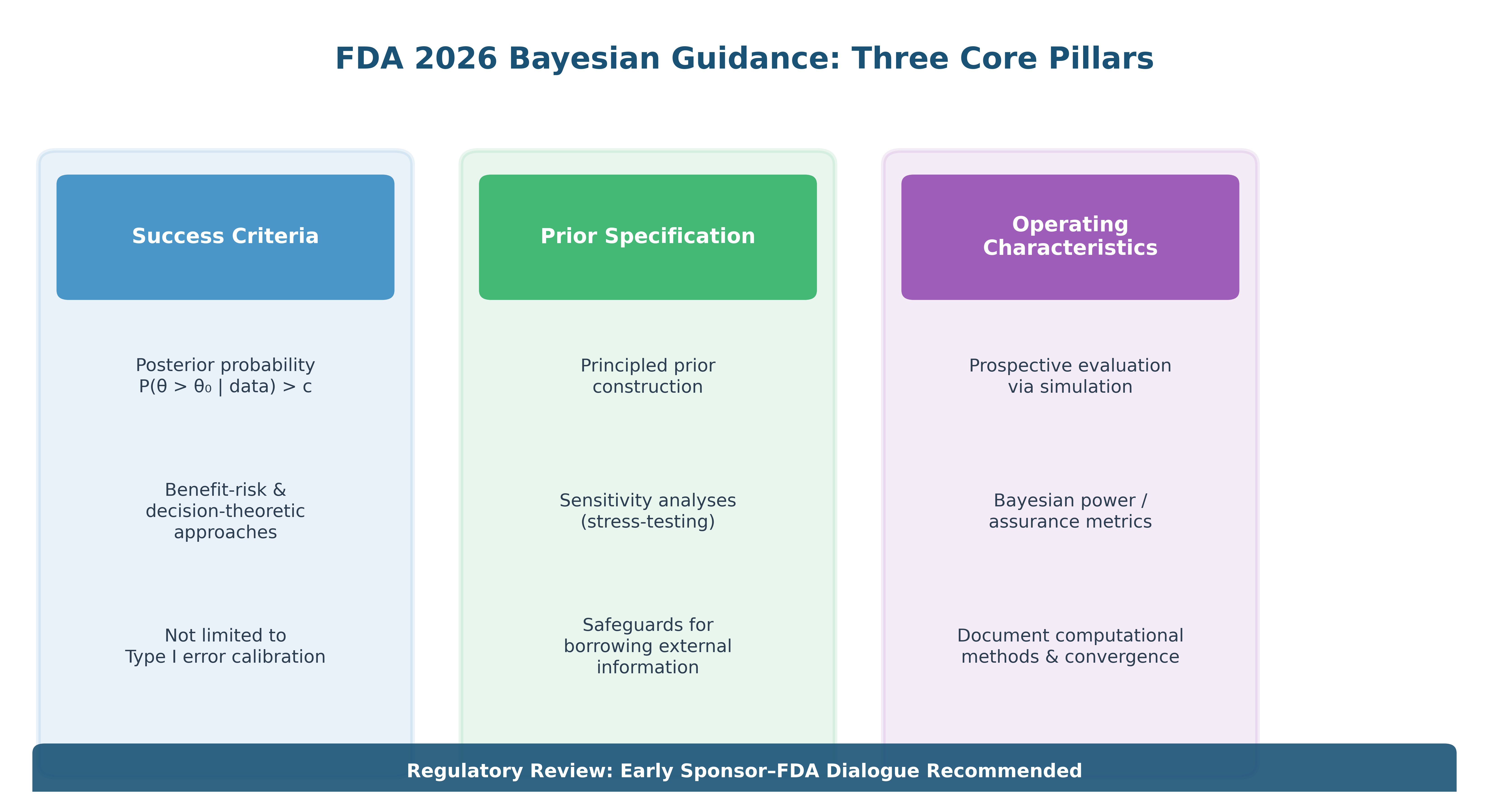
7.2 Success Criteria Under the Bayesian Framework
The guidance defines Bayesian success criteria through posterior probabilities:
\[ P(\theta > \theta_0 \mid \text{data}, \text{prior}) > c \]
where \(\theta\) is the treatment effect parameter, \(\theta_0\) is the null value, and \(c\) is the required posterior probability level.
The guidance allows calibrating \(c\) to control frequentist error rates. This is the most conservative approach — but Harrell warns this creates conceptual confusion by “wedding” Bayesian and frequentist thinking.
When sponsor and FDA agree, designs may target Bayesian operating metrics:
- Bayesian power (assurance): Average power over a design prior distribution
- Probability of correct decision: Weighted over plausible treatment effects
The most “Bayesian” option: assess the potential negative consequences of approving an ineffective drug or of not approving an effective drug. This framework acknowledges that both types of errors have costs.
7.3 Prior Distribution Specification
Show code
library(ggplot2)

x <- seq(-1.5, 1.0, length.out = 500)

# Priors for log(HR)
priors <- data.frame(
  x = rep(x, 4),
  density = c(
    dnorm(x, 0, 10),          # Non-informative (very flat)
    dnorm(x, 0, 0.5),         # Skeptical
    dnorm(x, -0.3, 0.3),      # Enthusiastic (centered on modest benefit)
    dnorm(x, -0.2, 0.15)      # Strong informative (from prior trials)
  ),
  prior_type = rep(c("Non-informative (σ = 10)",
                      "Skeptical (σ = 0.5)",
                      "Moderately enthusiastic (μ = -0.3)",
                      "Strong informative (prior trials)"), each = length(x))
)

# Observed data: log(HR) = -0.35, SE = 0.12
obs_mean <- -0.35
obs_se <- 0.12
likelihood <- dnorm(x, obs_mean, obs_se)

# Compute posteriors
compute_posterior <- function(prior_mean, prior_sd) {
  post_var <- 1 / (1/prior_sd^2 + 1/obs_se^2)
  post_mean <- post_var * (prior_mean/prior_sd^2 + obs_mean/obs_se^2)
  post_sd <- sqrt(post_var)
  dnorm(x, post_mean, post_sd)
}

posteriors <- data.frame(
  x = rep(x, 4),
  density = c(
    compute_posterior(0, 10),
    compute_posterior(0, 0.5),
    compute_posterior(-0.3, 0.3),
    compute_posterior(-0.2, 0.15)
  ),
  prior_type = rep(c("Non-informative (σ = 10)",
                      "Skeptical (σ = 0.5)",
                      "Moderately enthusiastic (μ = -0.3)",
                      "Strong informative (prior trials)"), each = length(x))
)

pal <- c("Non-informative (σ = 10)" = "#95a5a6",
         "Skeptical (σ = 0.5)" = "#e74c3c",
         "Moderately enthusiastic (μ = -0.3)" = "#2e86c1",
         "Strong informative (prior trials)" = "#27ae60")

p_prior <- ggplot(priors, aes(x = x, y = density, color = prior_type)) +
  geom_line(linewidth = 1.2) +
  geom_vline(xintercept = 0, linetype = "dashed", color = "grey50") +
  scale_color_manual(values = pal) +
  coord_cartesian(ylim = c(0, 3.5)) +
  labs(x = "log(Hazard Ratio)", y = "Density", title = "Prior Distributions",
       color = "Prior") +
  annotate("text", x = 0.05, y = 3.3, label = "No effect", size = 3, hjust = 0, color = "grey50") +
  annotate("text", x = -1.2, y = 3.3, label = "← Favors treatment", size = 3, color = "#1a5276") +
  theme_minimal(base_size = 11) +
  theme(plot.title = element_text(face = "bold", color = "#1a5276"),
        legend.position = "none")

p_post <- ggplot(posteriors, aes(x = x, y = density, color = prior_type)) +
  geom_line(linewidth = 1.2) +
  geom_vline(xintercept = 0, linetype = "dashed", color = "grey50") +
  geom_vline(xintercept = obs_mean, linetype = "dotted", color = "grey30") +
  annotate("text", x = obs_mean + 0.03, y = max(posteriors$density) * 0.95,
           label = paste0("Observed\nlog(HR)=", obs_mean), size = 3, hjust = 0) +
  scale_color_manual(values = pal) +
  labs(x = "log(Hazard Ratio)", y = "Density", title = "Posterior Distributions",
       subtitle = "Same data (log(HR) = -0.35, SE = 0.12), different priors",
       color = "Prior specification") +
  theme_minimal(base_size = 11) +
  theme(plot.title = element_text(face = "bold", color = "#1a5276"),
        plot.subtitle = element_text(color = "#7f8c8d"),
        legend.position = "bottom",
        legend.text = element_text(size = 9))

library(patchwork)
p_prior / p_post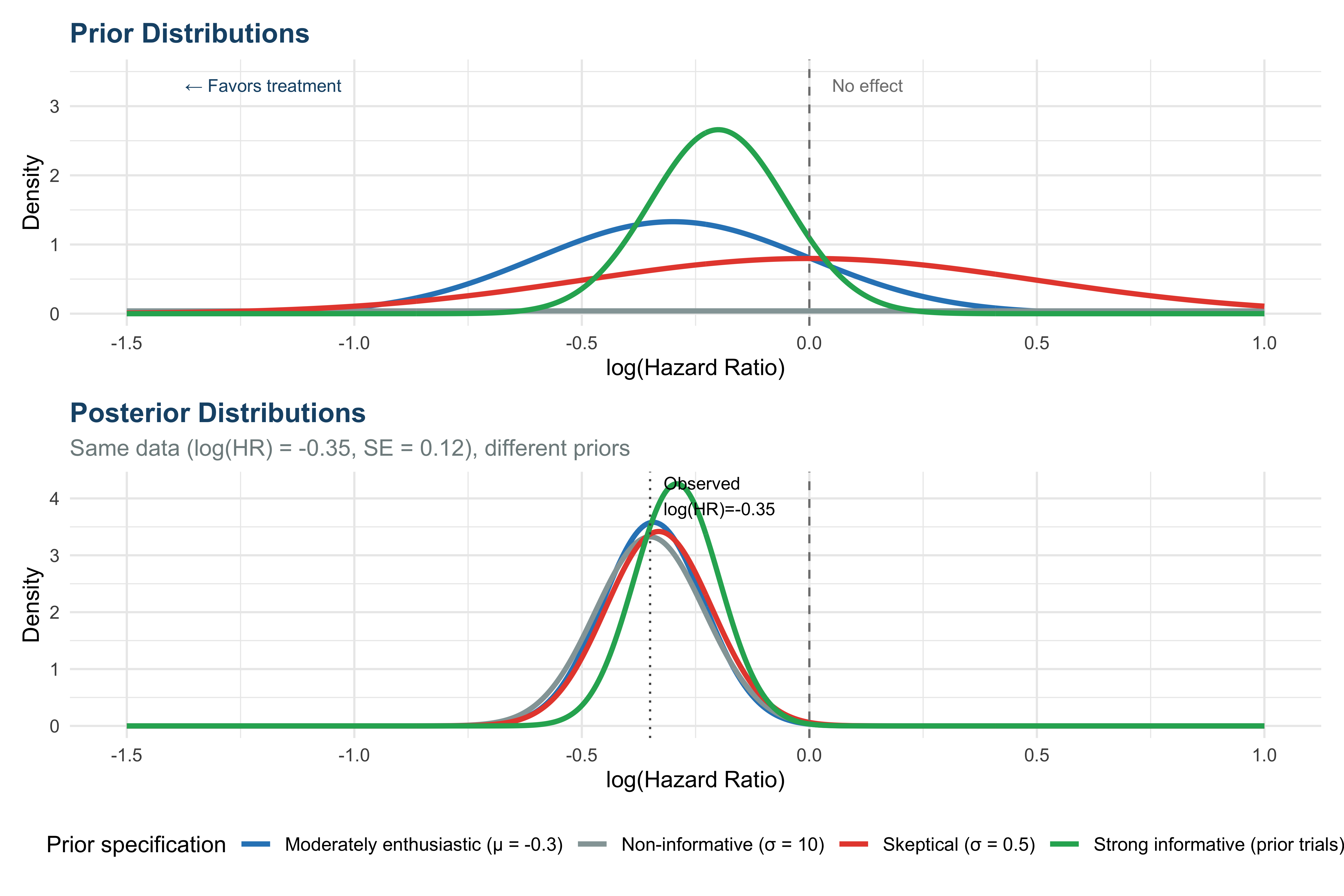
7.3.1 Key Insight: Priors Make Assumptions Explicit
Harrell emphasizes: “Disagreements about priors are surfaced and can be evaluated via sensitivity analyses, whereas implicit assumptions in frequentist planning can be harder to identify and quantify.” The FDA guidance requires sponsors to justify their prior choice and provide sensitivity analyses.
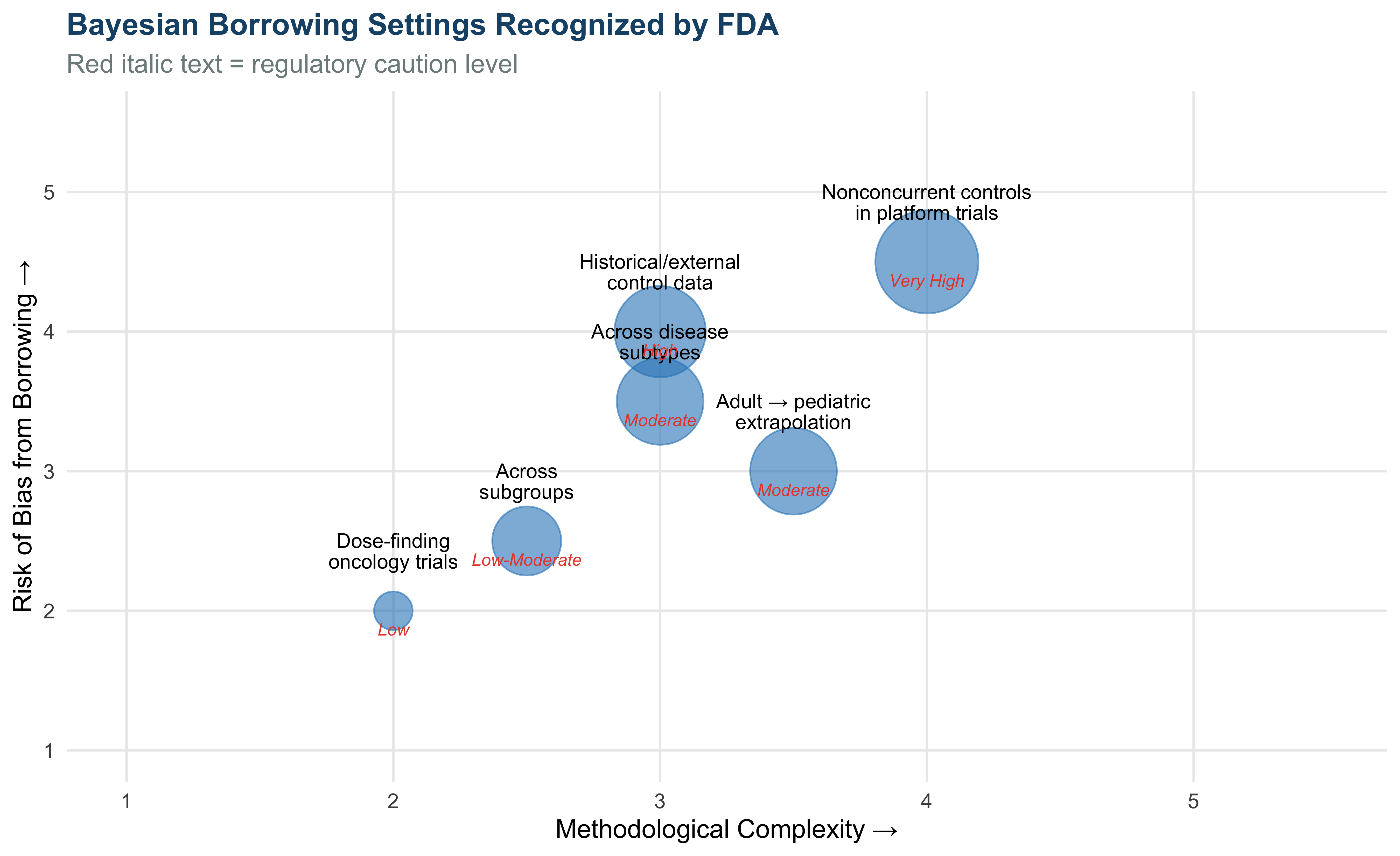
7.4 Borrowing External Information
The guidance outlines several settings where informative priors can borrow external data:
Show code
library(ggplot2)

borrowing <- data.frame(
  setting = c(
    "Historical/external\ncontrol data",
    "Nonconcurrent controls\nin platform trials",
    "Adult → pediatric\nextrapolation",
    "Across disease\nsubtypes",
    "Across\nsubgroups",
    "Dose-finding\noncology trials"
  ),
  complexity = c(3, 4, 3.5, 3, 2.5, 2),
  risk_of_bias = c(4, 4.5, 3, 3.5, 2.5, 2),
  regulatory_caution = c("High", "Very High", "Moderate", "Moderate", "Low-Moderate", "Low")
)

ggplot(borrowing, aes(x = complexity, y = risk_of_bias)) +
  geom_point(aes(size = complexity + risk_of_bias), color = "#2e86c1", alpha = 0.6) +
  geom_text(aes(label = setting), vjust = -1.2, size = 3.3, lineheight = 0.85) +
  geom_text(aes(label = regulatory_caution), vjust = 2, size = 2.8,
            color = "#e74c3c", fontface = "italic") +
  scale_size_continuous(range = c(8, 22), guide = "none") +
  scale_x_continuous(limits = c(1, 5.5)) +
  scale_y_continuous(limits = c(1, 5.5)) +
  labs(x = "Methodological Complexity →",
       y = "Risk of Bias from Borrowing →",
       title = "Bayesian Borrowing Settings Recognized by FDA",
       subtitle = "Red italic text = regulatory caution level") +
  theme_minimal(base_size = 12) +
  theme(
    plot.title = element_text(face = "bold", color = "#1a5276", size = 14),
    plot.subtitle = element_text(color = "#7f8c8d"),
    panel.grid.minor = element_blank()
  )
8 The Bayesian Time Machine and Platform Trials
8.1 Saville et al. (2022): The Proposal
The Bayesian Time Machine (Saville et al., Clinical Trials 2022) — a paper directly cited by the FDA guidance — proposes time-adjusted analyses to model temporal drift in multi-arm platform trials. This allows incorporation of nonconcurrent controls alongside concurrent ones.
Show code
import numpy as np
import matplotlib.pyplot as plt
import matplotlib.patches as mpatches

fig, ax = plt.subplots(figsize=(11, 5.5))

# Allocation scheme based on Senn's description of Saville et al.
# Rows: Arms (Control, Arm1-5), Cols: Periods 1-10
allocation = {
    'Control':  [50, 50, 33, 33, 33, 25, 25, 25, 25, 50],
    'Arm 1':    [50, 50, 33, 33,  0,  0,  0,  0,  0,  0],
    'Arm 2':    [ 0,  0, 33, 33, 33, 25,  0,  0,  0,  0],
    'Arm 3':    [ 0,  0,  0,  0, 33, 25, 25, 25,  0,  0],
    'Arm 4':    [ 0,  0,  0,  0, 33, 25, 25, 25,  0,  0],
    'Arm 5':    [ 0,  0,  0,  0,  0,  0, 25, 25, 25, 50],
}

colors = {
    'Control': '#34495e',
    'Arm 1': '#e74c3c',
    'Arm 2': '#2e86c1',
    'Arm 3': '#27ae60',
    'Arm 4': '#f39c12',
    'Arm 5': '#8e44ad'
}

arms = list(allocation.keys())
periods = range(1, 11)

for i, arm in enumerate(arms):
    for j, period in enumerate(periods):
        n = allocation[arm][j]
        if n > 0:
            rect = plt.Rectangle((j + 0.55, len(arms) - i - 0.65), 0.9, 0.7,
                                  facecolor=colors[arm], alpha=0.75,
                                  edgecolor='white', linewidth=1.5)
            ax.add_patch(rect)
            ax.text(j + 1, len(arms) - i - 0.3, str(n),
                    ha='center', va='center', fontsize=9,
                    fontweight='bold', color='white')

ax.set_xlim(0.4, 10.6)
(0.4, 10.6)Show code
ax.set_ylim(-0.2, len(arms) + 0.3)(-0.2, 6.3)Show code
ax.set_xticks(range(1, 11))
ax.set_xticklabels([f'Period {i}' for i in range(1, 11)], fontsize=9, rotation=45, ha='right')
ax.set_yticks([len(arms) - i - 0.3 for i in range(len(arms))])
ax.set_yticklabels(arms, fontsize=10)
ax.set_xlabel('Time Period', fontsize=12)
ax.set_title('Hypothetical Platform Trial Allocation\n(Based on Saville et al. 2022, as analyzed by Senn 2026)',
             fontsize=13, fontweight='bold', color='#1a5276')

# Annotation
ax.annotate('Arms 3 & 4 have\nnearly identical\ntiming', xy=(6, 2.2), fontsize=8,
            color='#7f8c8d', fontstyle='italic', ha='center')
ax.annotate('Arm 1 exits Period 4\nbut variance continues\nto decrease', xy=(5, 4.7),
            fontsize=8, color='#7f8c8d', fontstyle='italic', ha='center')

ax.spines['top'].set_visible(False)
ax.spines['right'].set_visible(False)

plt.tight_layout()
plt.savefig('platform_allocation.png', dpi=300, bbox_inches='tight')
plt.show()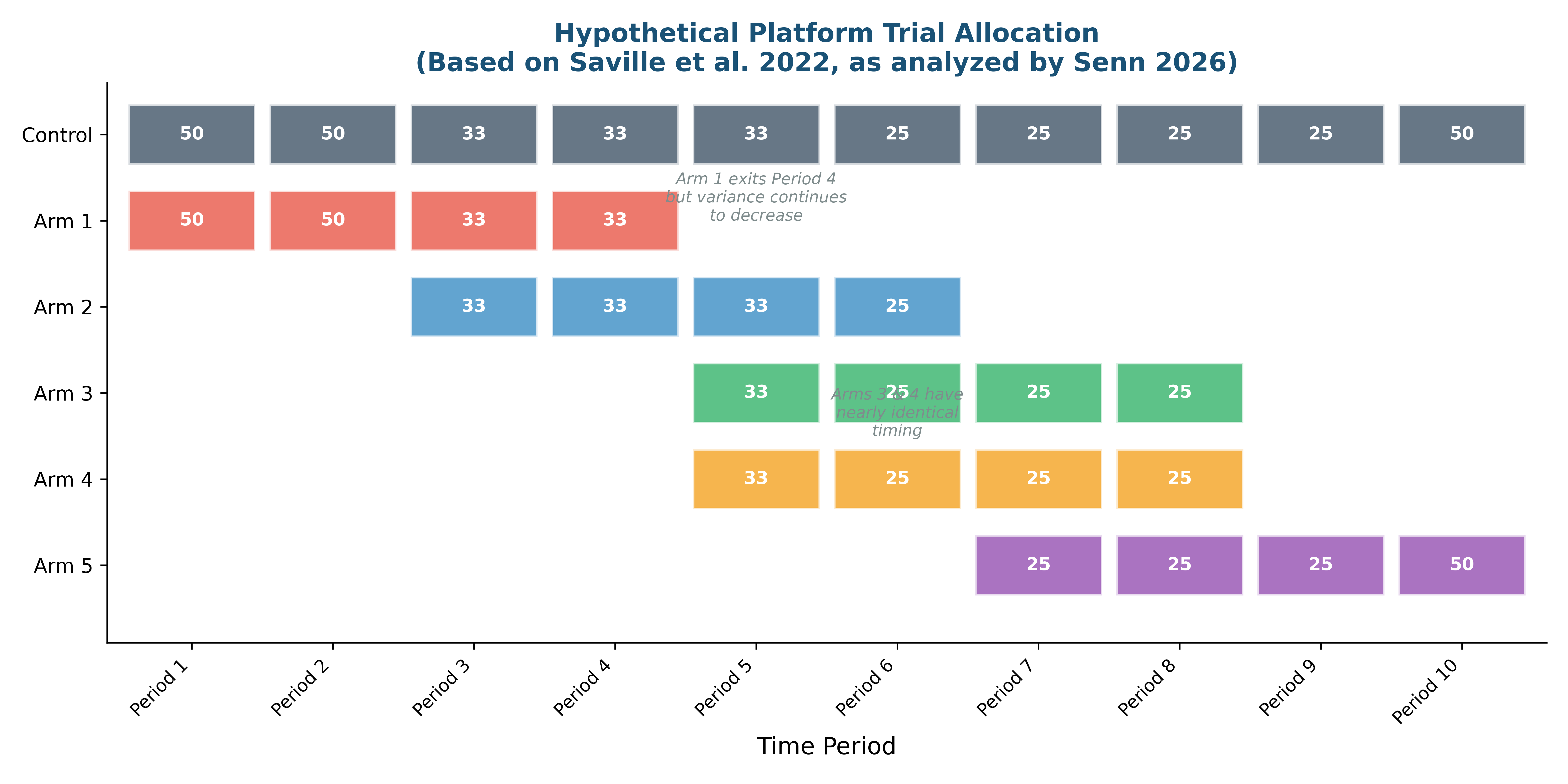
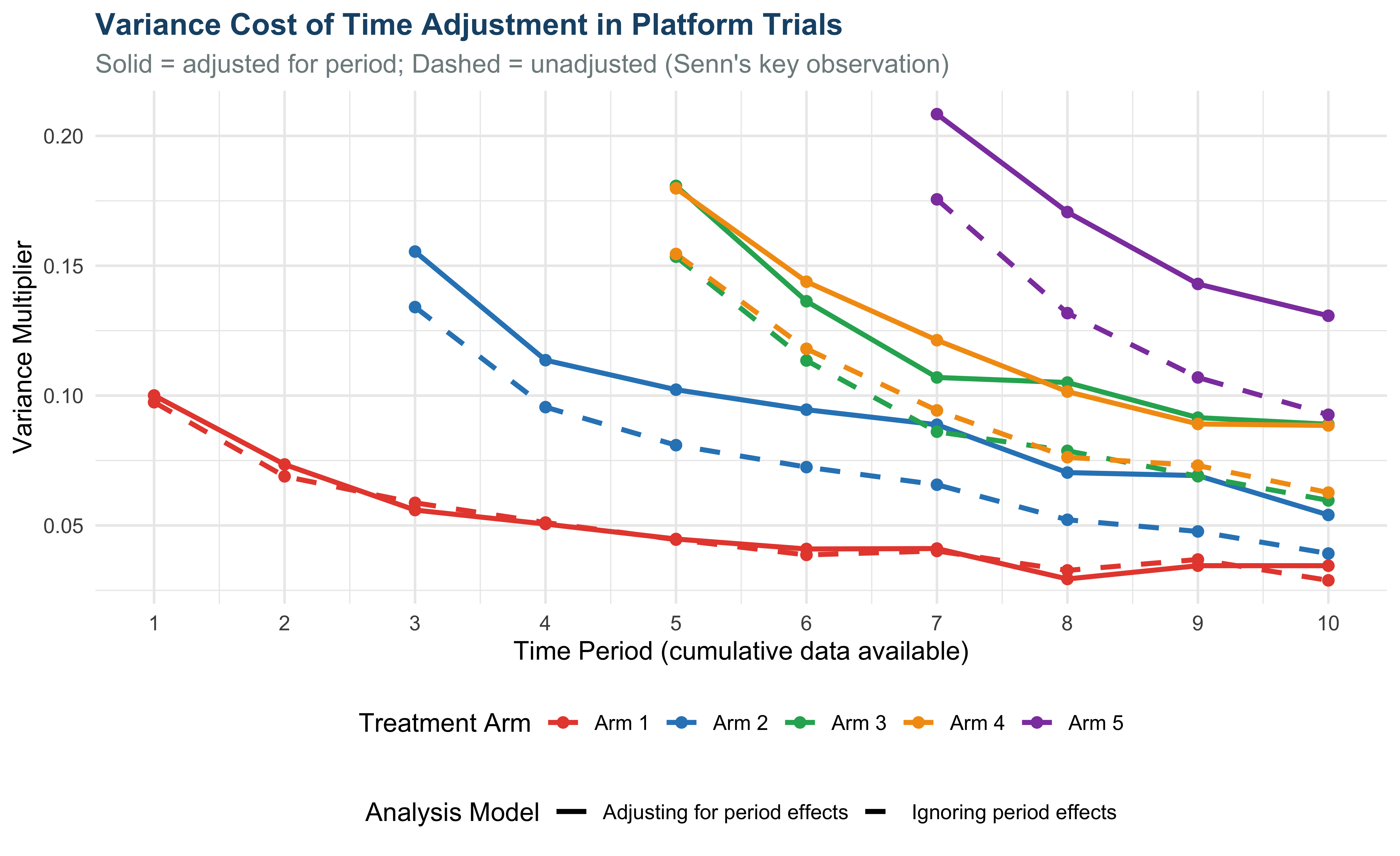
8.2 Variance Multipliers: The Cost of Adjusting for Time
Show code
library(ggplot2)

# Simulated variance multipliers based on Senn's description
# These are illustrative of the pattern described in the paper
periods_avail <- list(
  "Arm 1" = 1:10,
  "Arm 2" = 3:10,
  "Arm 3" = 5:10,
  "Arm 4" = 5:10,
  "Arm 5" = 7:10
)

set.seed(42)
df_vm <- data.frame()
for (arm in names(periods_avail)) {
  pds <- periods_avail[[arm]]
  n <- length(pds)

  # Unadjusted: decreasing with more data, lower baseline
  base_unadj <- ifelse(arm == "Arm 1", 0.04,
                 ifelse(arm == "Arm 2", 0.06,
                 ifelse(arm %in% c("Arm 3", "Arm 4"), 0.07, 0.08)))
  vm_unadj <- base_unadj / (seq_along(pds) * 0.18 + 0.3) + 0.01 +
    rnorm(n, 0, 0.003)

  # Adjusted: higher than unadjusted, especially for arms with less overlap
  # Exception: Arm 1 periods 1-4 (balanced with control)
  penalty <- ifelse(arm == "Arm 1", 0.005,
              ifelse(arm == "Arm 2", 0.02,
              ifelse(arm %in% c("Arm 3", "Arm 4"), 0.025, 0.035)))
  if (arm == "Arm 1") {
    vm_adj <- c(vm_unadj[1:4], vm_unadj[5:n] + penalty * seq_len(n-4)/n) +
      rnorm(n, 0, 0.002)
  } else {
    vm_adj <- vm_unadj + penalty + rnorm(n, 0, 0.003)
  }

  df_vm <- rbind(df_vm, data.frame(
    period = rep(pds, 2),
    vm = c(vm_unadj, vm_adj),
    arm = arm,
    model = rep(c("Ignoring period effects", "Adjusting for period effects"), each = n)
  ))
}

pal_arms <- c("Arm 1" = "#e74c3c", "Arm 2" = "#2e86c1", "Arm 3" = "#27ae60",
              "Arm 4" = "#f39c12", "Arm 5" = "#8e44ad")

ggplot(df_vm, aes(x = period, y = vm, color = arm, linetype = model)) +
  geom_line(linewidth = 1.1) +
  geom_point(size = 2) +
  scale_color_manual(values = pal_arms) +
  scale_linetype_manual(values = c("Ignoring period effects" = "dashed",
                                    "Adjusting for period effects" = "solid")) +
  scale_x_continuous(breaks = 1:10) +
  labs(x = "Time Period (cumulative data available)",
       y = "Variance Multiplier",
       title = "Variance Cost of Time Adjustment in Platform Trials",
       subtitle = "Solid = adjusted for period; Dashed = unadjusted (Senn's key observation)",
       color = "Treatment Arm", linetype = "Analysis Model") +
  theme_minimal(base_size = 12) +
  theme(
    plot.title = element_text(face = "bold", color = "#1a5276", size = 14),
    plot.subtitle = element_text(color = "#7f8c8d"),
    legend.position = "bottom",
    legend.box = "vertical"
  )
9 Stephen Senn’s Critique: “Beware of the Morlocks”
9.0.1 About the Critique
Stephen Senn, a distinguished statistical consultant, published “Beware of the Morlocks” in March 2026 — a pointed critique of the Bayesian Time Machine and what he terms “debased Bayes” and “debayesed Bayes” promoted by uncritical enthusiasm around the FDA guidance.
The title references H.G. Wells’s The Time Machine, where the Morlocks are the hidden dangers lurking beneath a seemingly pleasant surface.
“It sounds plausible enough tonight,” said the Medical Man; “but wait until tomorrow. Wait for the common sense of the morning.” ::: {.attribution} — H.G. Wells, The Time Machine, Ch. II (quoted by Senn)
:::
9.1 Senn’s Three Core Arguments
Show code
import matplotlib.pyplot as plt
import matplotlib.patches as mpatches

fig, ax = plt.subplots(figsize=(11, 7))
ax.set_xlim(0, 12)
(0.0, 12.0)Show code
ax.set_ylim(0, 10)(0.0, 10.0)Show code
ax.axis('off')(np.float64(0.0), np.float64(12.0), np.float64(0.0), np.float64(10.0))Show code
# Title
ax.text(6, 9.5, "Senn's Critique: Three Core Arguments", fontsize=16,
        fontweight='bold', ha='center', color='#8e44ad')

arguments = [
    {
        'y': 7.2, 'color': '#c0392b',
        'number': '1',
        'title': 'The Concurrent Control Problem',
        'body': (
            "Adjusting for time period effects is necessary to\n"
            "eliminate temporal drift bias, but this adjustment\n"
            "substantially INCREASES variance multipliers.\n\n"
            "You cannot compare Arm 3 to Arm 1 directly — there\n"
            "is no time period in which both are given. Indirect\n"
            "comparisons through control inflate variance."
        )
    },
    {
        'y': 4.2, 'color': '#2c3e50',
        'number': '2',
        'title': 'The Blinding / "Veiled Trial" Problem',
        'body': (
            "Saville et al. claim nonconcurrent controls differ\n"
            "only by time. Senn argues this is NOT TRUE.\n\n"
            "Platform trials with multiple arms require separate\n"
            "placebos per arm (veiled design). This creates not\n"
            "10 but potentially 24+ categories — with far higher\n"
            "variance than claimed."
        )
    },
    {
        'y': 1.2, 'color': '#8e44ad',
        'number': '3',
        'title': 'Administrative ≠ Statistical Efficiency',
        'body': (
            '"The principle values of adaptive designs are\n'
            'administrative efficiency and the ability to react\n'
            'swiftly to abandon unpromising treatments.\n'
            'Any claims beyond this should be viewed with\n'
            'suspicion." — Senn 2026\n\n'
            'Some hype is "not only ludicrous but dangerous."'
        )
    }
]

for arg in arguments:
    # Background box
    rect = mpatches.FancyBboxPatch((0.5, arg['y'] - 0.8), 11, 2.6,
                                     boxstyle="round,pad=0.2",
                                     facecolor=arg['color'], alpha=0.06,
                                     edgecolor=arg['color'], linewidth=2)
    ax.add_patch(rect)

    # Number circle
    circle = plt.Circle((1.5, arg['y'] + 0.5), 0.5, color=arg['color'], alpha=0.85)
    ax.add_patch(circle)
    ax.text(1.5, arg['y'] + 0.5, arg['number'], fontsize=18, fontweight='bold',
            color='white', ha='center', va='center')

    # Title
    ax.text(2.5, arg['y'] + 1.3, arg['title'], fontsize=13, fontweight='bold',
            color=arg['color'])

    # Body
    ax.text(2.5, arg['y'] + 0.8, arg['body'], fontsize=9.5, color='#2c3e50',
            va='top', linespacing=1.3, family='monospace')

plt.tight_layout()
plt.savefig('senn_arguments.png', dpi=300, bbox_inches='tight')
plt.show()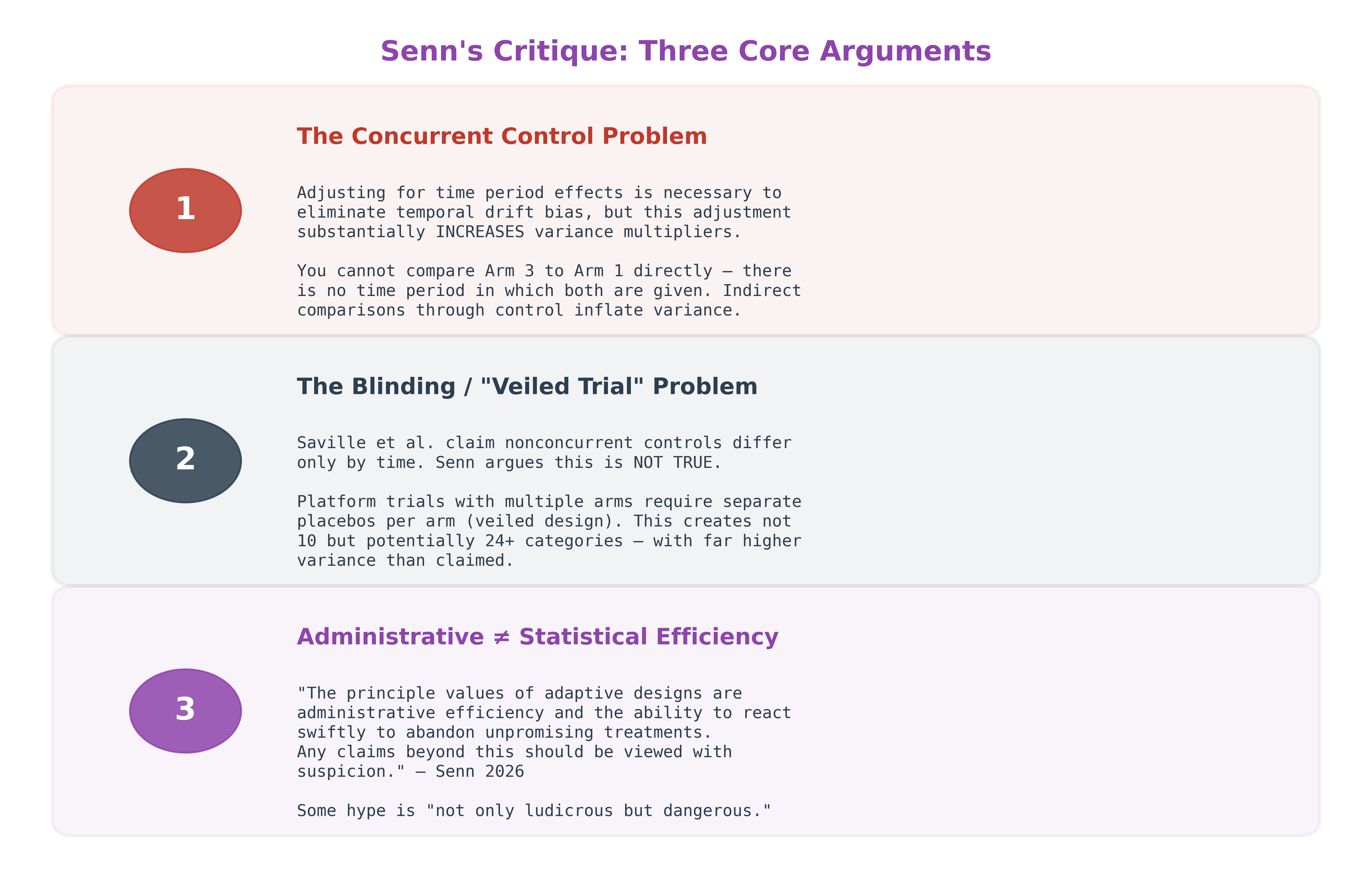
9.2 The Veiled Trial Problem: An Overlooked Threat
Senn introduces a critical and often overlooked concept: veiled trials.
A veiled trial is one where patients do not know which treatment they are receiving, but do know of at least one treatment in the trial they are NOT receiving. This is common in platform trials with different modes of administration or dosing.
If blinding matters — and it usually does — then each active treatment in a platform trial requires its own control. In the Saville et al. design:
- Without veiling consideration: 10 period categories
- With veiling consideration: Up to 24 placebo-and-time categories
The resulting variance multipliers would be substantially higher than Saville et al. report.
Consider a platform trial in AML testing:
- Oral menin inhibitor (revumenib)
- IV antibody-drug conjugate (gemtuzumab)
- Subcutaneous hypomethylating agent (azacitidine)
Even with placebo matching, patients can infer their likely arm from route of administration, creating differential expectation effects that violate the exchangeability assumption across time periods.
9.3 The Center-Drift Problem
Show code
library(ggplot2)

set.seed(123)
n_centers <- 12
n_periods <- 10

# Simulate center activity
center_start <- c(1,1,1,1,2,2,3,4,5,6,7,8)
center_end <- c(10,10,8,6,10,10,10,10,10,10,10,10)

df_centers <- data.frame()
for (i in 1:n_centers) {
  active_periods <- center_start[i]:center_end[i]
  df_centers <- rbind(df_centers, data.frame(
    center = paste0("Site ", LETTERS[i]),
    period = active_periods,
    center_id = i
  ))
}

df_centers$active <- 1

ggplot(df_centers, aes(x = period, y = reorder(center, -center_id), fill = factor(center_id))) +
  geom_tile(width = 0.85, height = 0.85, alpha = 0.8, show.legend = FALSE) +
  geom_vline(xintercept = c(3.5, 6.5), linetype = "dashed", color = "#e74c3c", linewidth = 0.8) +
  annotate("text", x = 2, y = 13, label = "Arm 1\nenters", color = "#e74c3c",
           size = 3, fontface = "bold") +
  annotate("text", x = 5, y = 13, label = "Arm 2\nenters", color = "#e74c3c",
           size = 3, fontface = "bold") +
  scale_x_continuous(breaks = 1:10) +
  scale_fill_manual(values = rep(c("#2e86c1", "#3498db", "#5dade2", "#85c1e9",
                                     "#27ae60", "#2ecc71", "#58d68d", "#82e0aa",
                                     "#8e44ad", "#a569bd", "#bb8fce", "#d2b4de"), 1)) +
  labs(x = "Time Period", y = NULL,
       title = "Center Composition Drift in a Platform Trial",
       subtitle = "Senn warns: if allocation rules change when centers join/leave, concurrent control is compromised") +
  theme_minimal(base_size = 12) +
  theme(
    plot.title = element_text(face = "bold", color = "#1a5276", size = 14),
    plot.subtitle = element_text(color = "#7f8c8d", size = 10),
    panel.grid = element_blank()
  )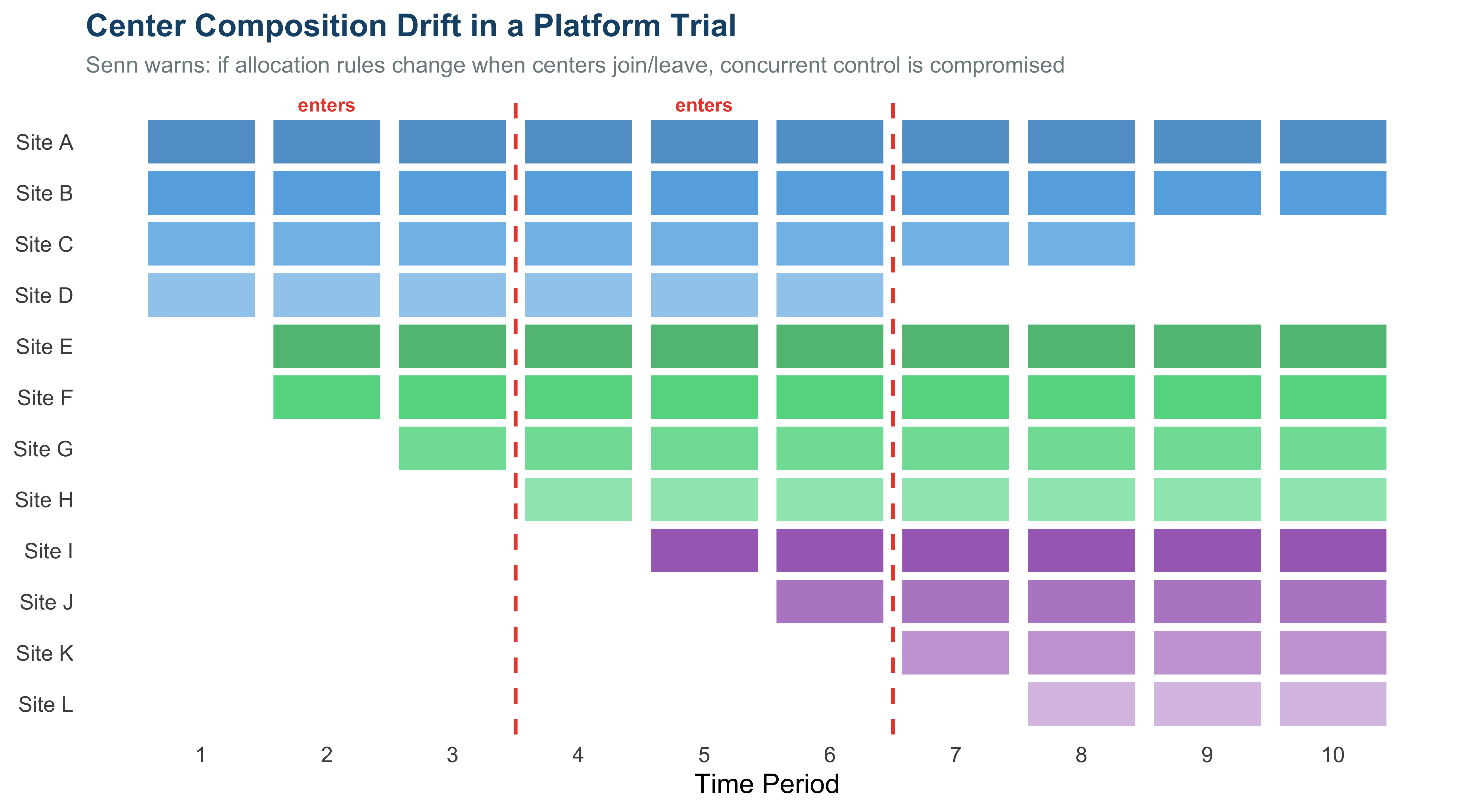
Senn has served on multiple Data Safety Monitoring Boards for trials with adaptive allocation ratios and found this “a challenging experience.” He notes that center heterogeneity creates confounding that no amount of statistical modeling can fully address — neither Bayesian nor frequentist.
10 Bayesian Sequential Monitoring: The Multiplicity Solution
10.1 Why Bayesian Methods Eliminate the Multiplicity Problem
Show code
library(ggplot2)

set.seed(2026)

# Simulate a trial with true HR = 0.75 (log HR = -0.29)
true_loghr <- -0.29
n_max <- 400
n_looks <- seq(50, n_max, by = 25)

# Simulate cumulative data
cum_loghr <- numeric(length(n_looks))
cum_se <- numeric(length(n_looks))
posterior_prob <- numeric(length(n_looks))
pval <- numeric(length(n_looks))

for (i in seq_along(n_looks)) {
  n <- n_looks[i]
  # Simulated observed log(HR) with noise that decreases with sample size
  cum_loghr[i] <- true_loghr + rnorm(1, 0, 0.5/sqrt(n))
  cum_se[i] <- 1/sqrt(n) * 2.5

  # Bayesian posterior: skeptical prior N(0, 0.35^2)
  prior_mean <- 0; prior_sd <- 0.35
  post_var <- 1/(1/prior_sd^2 + 1/cum_se[i]^2)
  post_mean <- post_var * (prior_mean/prior_sd^2 + cum_loghr[i]/cum_se[i]^2)
  post_sd <- sqrt(post_var)
  posterior_prob[i] <- pnorm(0, mean = post_mean, sd = post_sd) # P(logHR < 0)

  # Frequentist p-value
  z <- cum_loghr[i] / cum_se[i]
  pval[i] <- pnorm(z) # one-sided
}

df_seq <- data.frame(
  n = rep(n_looks, 2),
  value = c(posterior_prob, pval),
  metric = rep(c("Bayesian P(HR < 1 | data, prior)", "Frequentist p-value"), each = length(n_looks))
)

# O'Brien-Fleming adjusted alpha boundaries (approximate)
obf_alpha <- c(rep(0.00001, 3), rep(0.0005, 3), rep(0.005, 3), rep(0.015, 3), 0.025, 0.025, 0.025)

p1 <- ggplot(subset(df_seq, metric == "Bayesian P(HR < 1 | data, prior)"),
             aes(x = n, y = value)) +
  geom_line(color = "#27ae60", linewidth = 1.3) +
  geom_point(color = "#27ae60", size = 2.5) +
  geom_hline(yintercept = 0.95, linetype = "dashed", color = "#e74c3c") +
  geom_hline(yintercept = 0.975, linetype = "dotted", color = "#c0392b") +
  annotate("text", x = 380, y = 0.957, label = "Decision threshold\n(P = 0.95)", size = 3, color = "#e74c3c") +
  scale_y_continuous(limits = c(0.4, 1)) +
  labs(x = "Patients enrolled", y = "Posterior P(HR < 1)",
       title = "Bayesian: Smooth Update",
       subtitle = "Same threshold at every look — no penalty") +
  theme_minimal(base_size = 11) +
  theme(plot.title = element_text(face = "bold", color = "#1a6e4e"))

p2 <- ggplot(subset(df_seq, metric == "Frequentist p-value"),
             aes(x = n, y = value)) +
  geom_line(color = "#e74c3c", linewidth = 1.3) +
  geom_point(color = "#e74c3c", size = 2.5) +
  geom_step(data = data.frame(n = n_looks, alpha = obf_alpha[1:length(n_looks)]),
            aes(x = n, y = alpha), color = "#2e86c1", linewidth = 1, linetype = "dashed") +
  annotate("text", x = 350, y = 0.03, label = "OBF boundary\n(decreasing α)", size = 3, color = "#2e86c1") +
  scale_y_continuous(limits = c(0, 0.15)) +
  labs(x = "Patients enrolled", y = "p-value (one-sided)",
       title = "Frequentist: α-Spending Required",
       subtitle = "Must cross increasingly stringent boundaries") +
  theme_minimal(base_size = 11) +
  theme(plot.title = element_text(face = "bold", color = "#c0392b"))

library(patchwork)
p1 + p2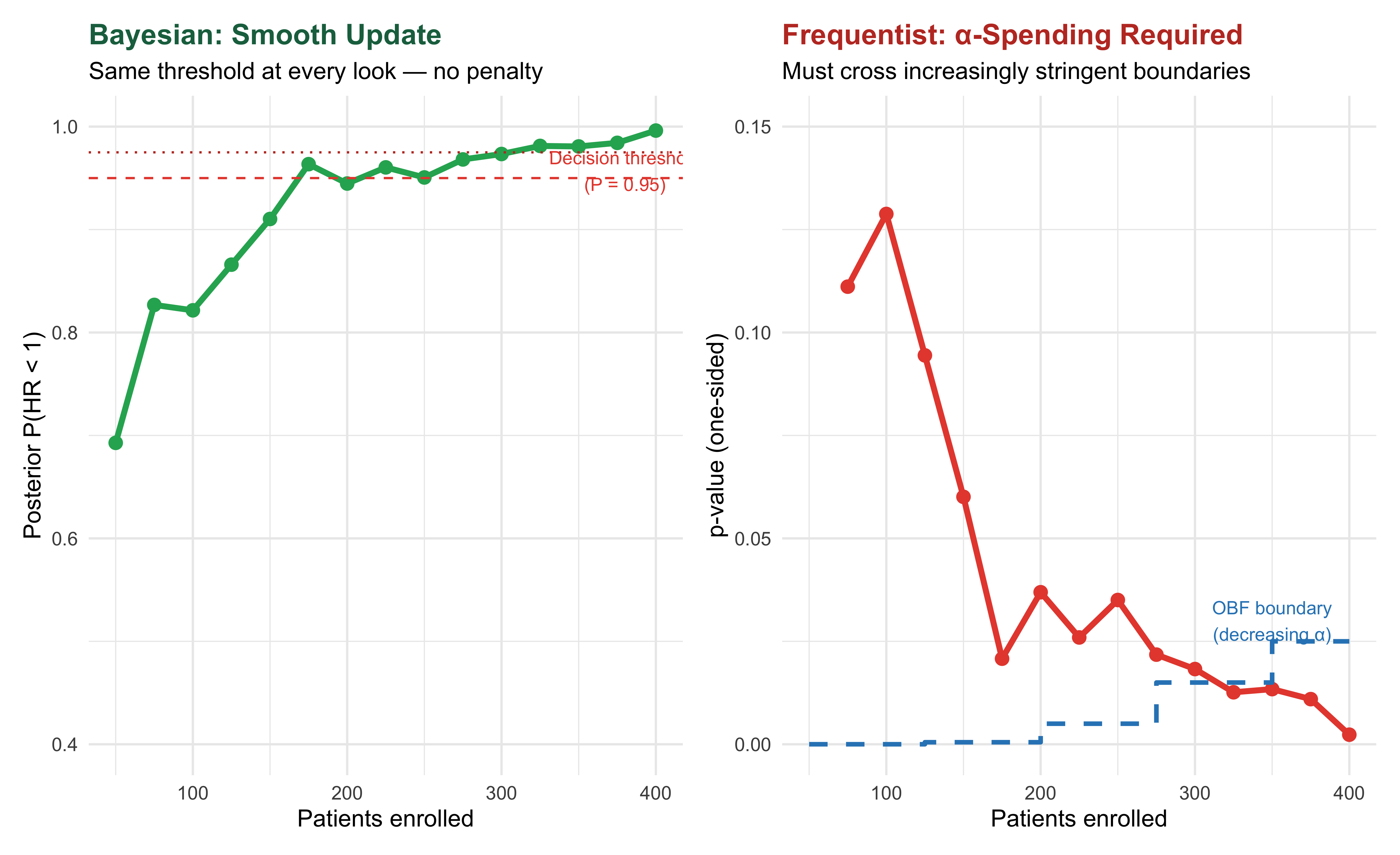
“In a Bayesian analysis, it is entirely appropriate to collect data until a point has been proven or disproven, or until the data collector runs out of time, money, or patience.” ::: {.attribution} — Edwards, Lindman, & Savage (1963), quoted by Harrell
:::
11 Practical Implications for Hematology-Oncology Trials
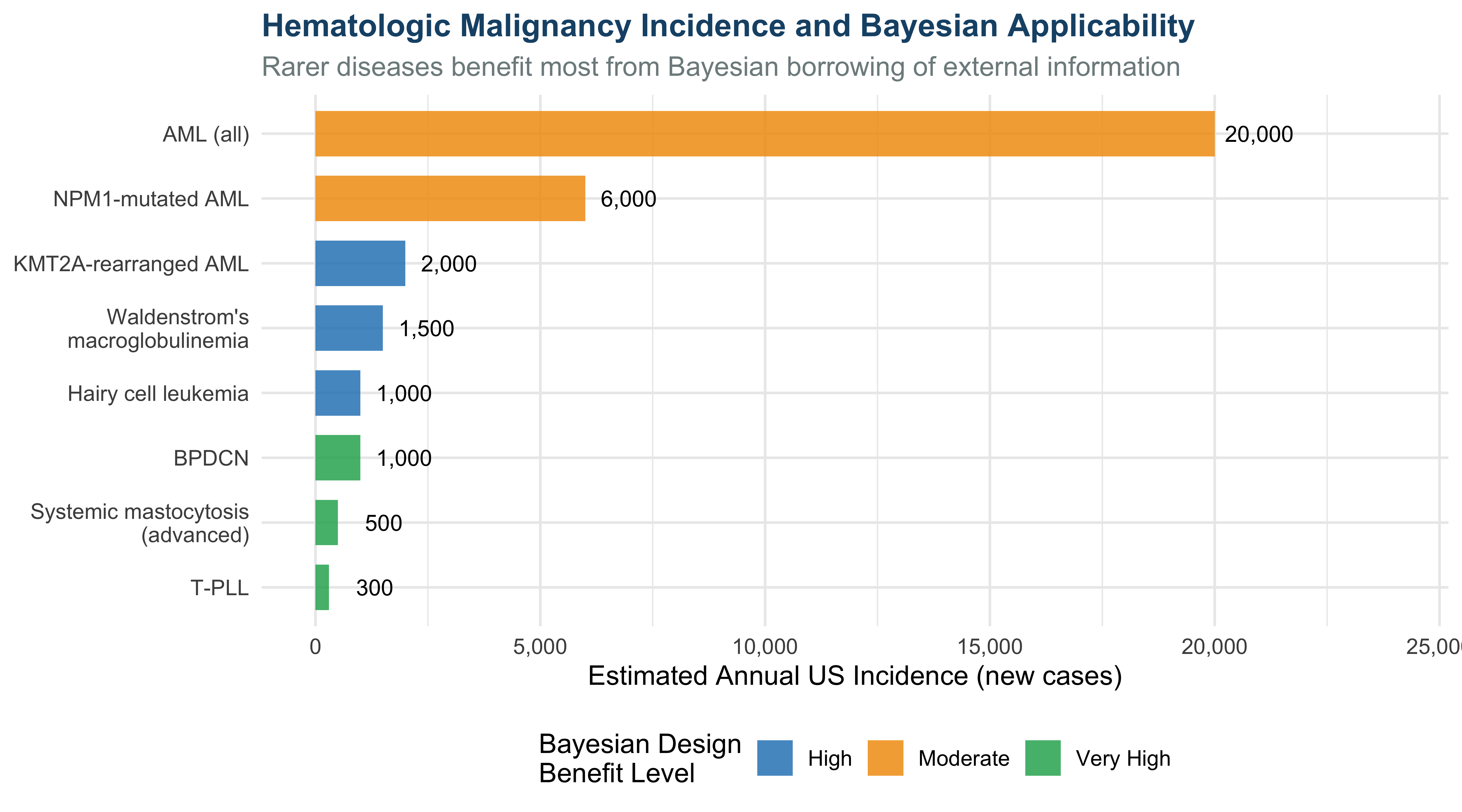
11.1 Rare Hematologic Malignancies: Where Bayesian Methods Shine
Show code
library(ggplot2)

diseases <- data.frame(
  disease = c(
    "AML (all)",
    "NPM1-mutated AML",
    "KMT2A-rearranged AML",
    "BPDCN",
    "T-PLL",
    "Hairy cell leukemia",
    "Systemic mastocytosis\n(advanced)",
    "Waldenstrom's\nmacroglobulinemia"
  ),
  incidence = c(20000, 6000, 2000, 1000, 300, 1000, 500, 1500),
  bayesian_benefit = c("Moderate", "Moderate", "High", "Very High",
                        "Very High", "High", "Very High", "High")
)

diseases$bayesian_color <- ifelse(diseases$bayesian_benefit == "Very High", "#27ae60",
                            ifelse(diseases$bayesian_benefit == "High", "#2e86c1", "#f39c12"))

ggplot(diseases, aes(x = reorder(disease, incidence), y = incidence, fill = bayesian_benefit)) +
  geom_col(width = 0.7, alpha = 0.85) +
  geom_text(aes(label = format(incidence, big.mark = ",")), hjust = -0.15, size = 3.5) +
  coord_flip() +
  scale_fill_manual(values = c("Moderate" = "#f39c12", "High" = "#2e86c1", "Very High" = "#27ae60"),
                    name = "Bayesian Design\nBenefit Level") +
  scale_y_continuous(limits = c(0, 24000), labels = scales::comma) +
  labs(x = NULL, y = "Estimated Annual US Incidence (new cases)",
       title = "Hematologic Malignancy Incidence and Bayesian Applicability",
       subtitle = "Rarer diseases benefit most from Bayesian borrowing of external information") +
  theme_minimal(base_size = 12) +
  theme(
    plot.title = element_text(face = "bold", color = "#1a5276", size = 14),
    plot.subtitle = element_text(color = "#7f8c8d"),
    legend.position = "bottom"
  )
11.2 Summary Comparison Table
Show code
library(knitr)

comparison <- data.frame(
  Feature = c(
    "Primary inferential framework",
    "Success criterion",
    "Multiplicity handling",
    "Prior information",
    "External data borrowing",
    "Sequential monitoring",
    "Treatment effect estimation",
    "Simulation requirements",
    "Type I error control",
    "Rare disease applicability",
    "Key limitation noted"
  ),
  `Adaptive_2019` = c(
    "Frequentist (primary); Bayesian acknowledged",
    "p < 0.025 (one-sided)",
    "α-spending functions (Lan-DeMets)",
    "Implicit in sample size assumptions",
    "Acknowledged but limited guidance",
    "Group sequential with stopping boundaries",
    "Bias-adjusted estimates (complex; rarely done)",
    "100,000 iterations per scenario",
    "Strict: must be ≤ 0.025",
    "Limited: minimum sample sizes expected",
    "Logistical complexity of maintaining integrity"
  ),
  `Bayesian_2026` = c(
    "Bayesian (primary); frequentist calibration optional",
    "P(θ > θ₀ | data) > c",
    "Not needed (posterior supersedes prior looks)",
    "Explicit prior distribution (justified & stress-tested)",
    "Detailed framework: historical, RWE, nonconcurrent",
    "Continuous monitoring; no α-penalty",
    "Posterior mean (naturally shrunk by prior if stopped early)",
    "May be needed for operating characteristics",
    "Optional; can use Bayesian operating metrics instead",
    "Strong: borrowing enables feasible designs",
    "Prior misspecification; computational complexity"
  )
)

names(comparison) <- c("Feature", "Adaptive Designs (2019)", "Bayesian Methodology (2026)")
kable(comparison, align = c("l", "l", "l"))| Feature | Adaptive Designs (2019) | Bayesian Methodology (2026) |
|---|---|---|
| Primary inferential framework | Frequentist (primary); Bayesian acknowledged | Bayesian (primary); frequentist calibration optional |
| Success criterion | p < 0.025 (one-sided) | P(θ > θ₀ | data) > c |
| Multiplicity handling | α-spending functions (Lan-DeMets) | Not needed (posterior supersedes prior looks) |
| Prior information | Implicit in sample size assumptions | Explicit prior distribution (justified & stress-tested) |
| External data borrowing | Acknowledged but limited guidance | Detailed framework: historical, RWE, nonconcurrent |
| Sequential monitoring | Group sequential with stopping boundaries | Continuous monitoring; no α-penalty |
| Treatment effect estimation | Bias-adjusted estimates (complex; rarely done) | Posterior mean (naturally shrunk by prior if stopped early) |
| Simulation requirements | 100,000 iterations per scenario | May be needed for operating characteristics |
| Type I error control | Strict: must be ≤ 0.025 | Optional; can use Bayesian operating metrics instead |
| Rare disease applicability | Limited: minimum sample sizes expected | Strong: borrowing enables feasible designs |
| Key limitation noted | Logistical complexity of maintaining integrity | Prior misspecification; computational complexity |
12 Synthesis: Points of Agreement and Tension
Show code
import matplotlib.pyplot as plt
import matplotlib.patches as mpatches
import numpy as np

fig, ax = plt.subplots(figsize=(11, 6.5))
ax.set_xlim(0, 12)
(0.0, 12.0)Show code
ax.set_ylim(0, 9)(0.0, 9.0)Show code
ax.axis('off')(np.float64(0.0), np.float64(12.0), np.float64(0.0), np.float64(9.0))Show code
ax.text(6, 8.6, 'Areas of Agreement and Tension', fontsize=16,
        fontweight='bold', ha='center', color='#1a5276')

# Agreement section
agree_box = mpatches.FancyBboxPatch((0.3, 5.5), 11.4, 2.8,
                                      boxstyle="round,pad=0.2",
                                      facecolor='#d5f5e3', alpha=0.5,
                                      edgecolor='#27ae60', linewidth=2)
ax.add_patch(agree_box)
ax.text(6, 8.0, '✓  ALL THREE AGREE', fontsize=12, fontweight='bold',
        ha='center', color='#1e8449')

agreements = [
    'Randomization and concurrent control remain the gold standard for causal inference',
    'Complete prespecification of trial design and analysis is essential',
    'Bayesian methods have genuine value, especially in rare diseases and pediatric trials',
    'Prior distributions must be justified, transparent, and stress-tested via sensitivity analysis',
    'Platform trials offer administrative efficiency — but statistical claims need scrutiny'
]
for i, txt in enumerate(agreements):
    ax.text(1.0, 7.5 - i*0.4, f'• {txt}', fontsize=9, color='#2c3e50')

# Tension section
tension_box = mpatches.FancyBboxPatch((0.3, 0.3), 11.4, 4.8,
                                        boxstyle="round,pad=0.2",
                                        facecolor='#fdedec', alpha=0.5,
                                        edgecolor='#e74c3c', linewidth=2)
ax.add_patch(tension_box)
ax.text(6, 4.8, '⚡ KEY TENSIONS', fontsize=12, fontweight='bold',
        ha='center', color='#c0392b')

tensions = [
    ('Should Bayesian designs be calibrated to\nType I error?',
     'Harrell: No — this creates hybrid mess',
     'FDA: Optional; Senn: Frequentist metrics\nstill have value'),
    ('Can the Bayesian Time Machine replace\nconcurrent control?',
     'FDA/Berry: Yes, with time adjustment',
     'Senn: No — veiled trials, center drift,\nvariance inflation'),
    ('Are adaptive platform trials statistically\nefficient?',
     'FDA/Berry: Yes — shared controls,\nborrowing',
     'Senn: Only administratively — statistical\nclaims are "ludicrous"'),
    ('How much external borrowing is safe?',
     'Harrell: Principled priors are transparent',
     'Senn: "Find out as much as possible about\nany data you intend to use"')
]

y_start = 4.3
for i, (question, left, right) in enumerate(tensions):
    y = y_start - i * 1.05
    ax.text(0.6, y, question, fontsize=8.5, fontweight='bold', color='#2c3e50',
            va='top', linespacing=1.2)
    ax.text(5.5, y, left, fontsize=8, color='#27ae60', va='top', linespacing=1.2)
    ax.text(8.8, y, right, fontsize=8, color='#c0392b', va='top', linespacing=1.2)

plt.tight_layout()
plt.savefig('synthesis.png', dpi=300, bbox_inches='tight')
plt.show()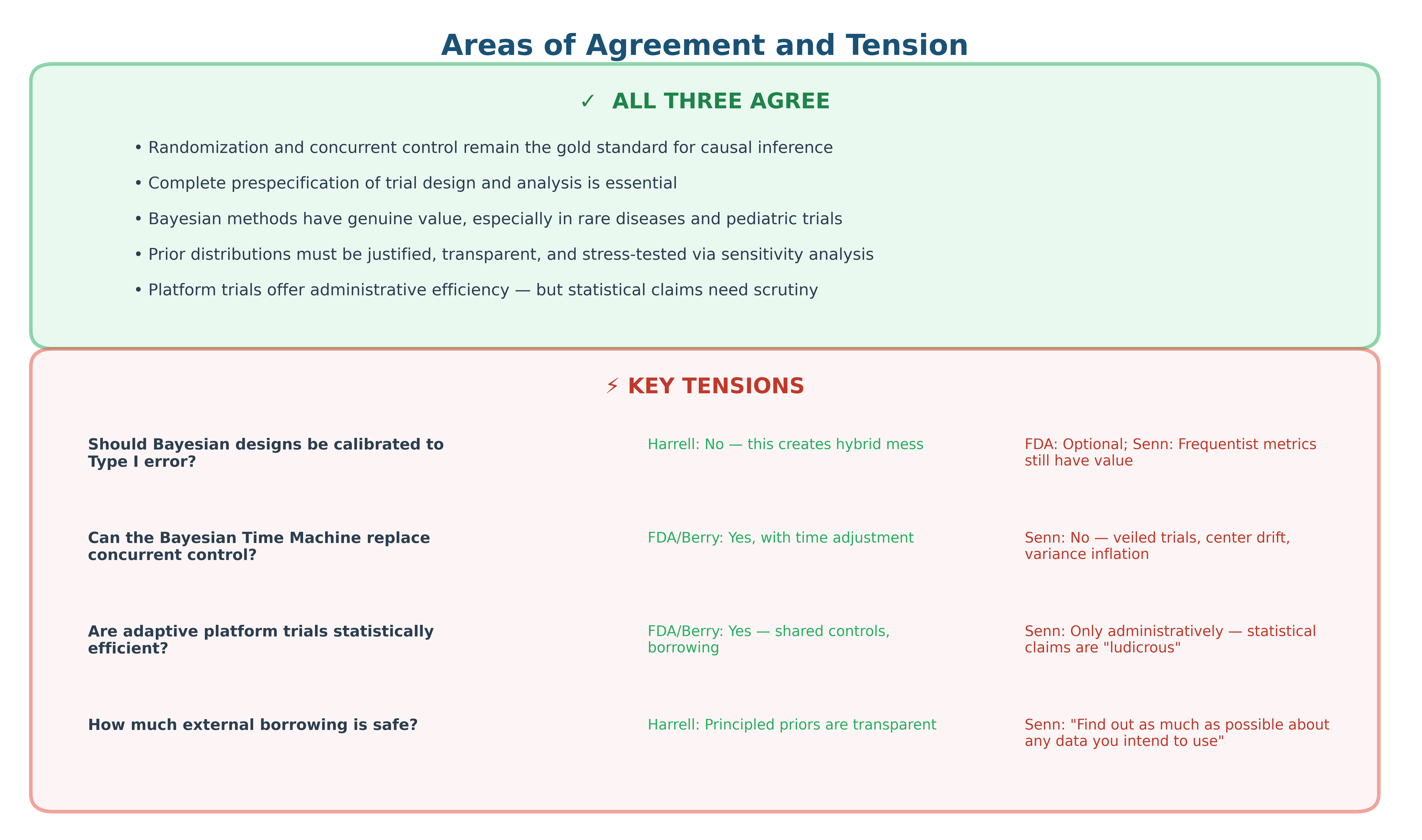
13 Recommendations for Trainees and Junior Faculty
13.0.1 Five Things Every Hematology-Oncology Fellow Should Know
A p-value of 0.04 doesn’t mean 96% probability the drug works. It means there’s a 4% chance of data this extreme if the drug has zero effect. The Bayesian posterior probability is what you actually want.
Early stopping inflates treatment effects. When trials stop early for efficacy, conventional estimates are biased upward. Bayesian skeptical priors naturally correct this.
Multiple endpoints don’t require multiple penalties (under Bayes). The agonizing debate over primary vs. secondary endpoints is a frequentist artifact.
Platform trials are administratively efficient but not necessarily statistically superior. Be skeptical of claims that borrowing nonconcurrent controls is “free” precision.
The prior is a feature, not a bug. Making assumptions explicit (through the prior) is more honest than hiding them (in sample size calculations, endpoint selection, and multiplicity adjustments).
13.1 Recommended Resources
rmsbpackage (Frank Harrell) — Bayesian regression modeling strategiesbrms— Bayesian regression models using Stanrstanarm— Applied regression modeling in Stanbayesplot— Visualization for Bayesian modelsRBesT— R Bayesian evidence synthesis tools (for borrowing)- Harrell’s course materials: hbiostat.org/R
PyMC— Probabilistic programmingArviZ— Bayesian visualization and diagnosticsbambi— Bayesian model building interfacecmdstanpy— Python interface to CmdStan
- Harrell FE. Statistical Thinking blog: fharrell.com
- Harrell FE. Regression Modeling Strategies (2nd ed., Springer)
- Senn SJ. Statistical Issues in Drug Development (3rd ed., Wiley)
- Berry SM et al. Bayesian Adaptive Methods for Clinical Trials (CRC Press)
- FDA Draft Guidance: regulations.gov, Docket FDA-2025-D-3217
14 Appendix: Technical Details
14.1 Bayesian Updating Formula
For a normal likelihood with known variance:
\[ \underbrace{p(\theta | y)}_{\text{posterior}} \propto \underbrace{p(y | \theta)}_{\text{likelihood}} \times \underbrace{p(\theta)}_{\text{prior}} \]
With conjugate normal prior \(\theta \sim N(\mu_0, \sigma_0^2)\) and data \(\bar{y} \sim N(\theta, \sigma^2/n)\):
\[ \theta | \bar{y} \sim N\left(\frac{\frac{\mu_0}{\sigma_0^2} + \frac{n\bar{y}}{\sigma^2}}{\frac{1}{\sigma_0^2} + \frac{n}{\sigma^2}}, \quad \frac{1}{\frac{1}{\sigma_0^2} + \frac{n}{\sigma^2}}\right) \]
The posterior precision equals the sum of the prior precision and the data precision — this is the mathematical basis for Bayesian “borrowing.”
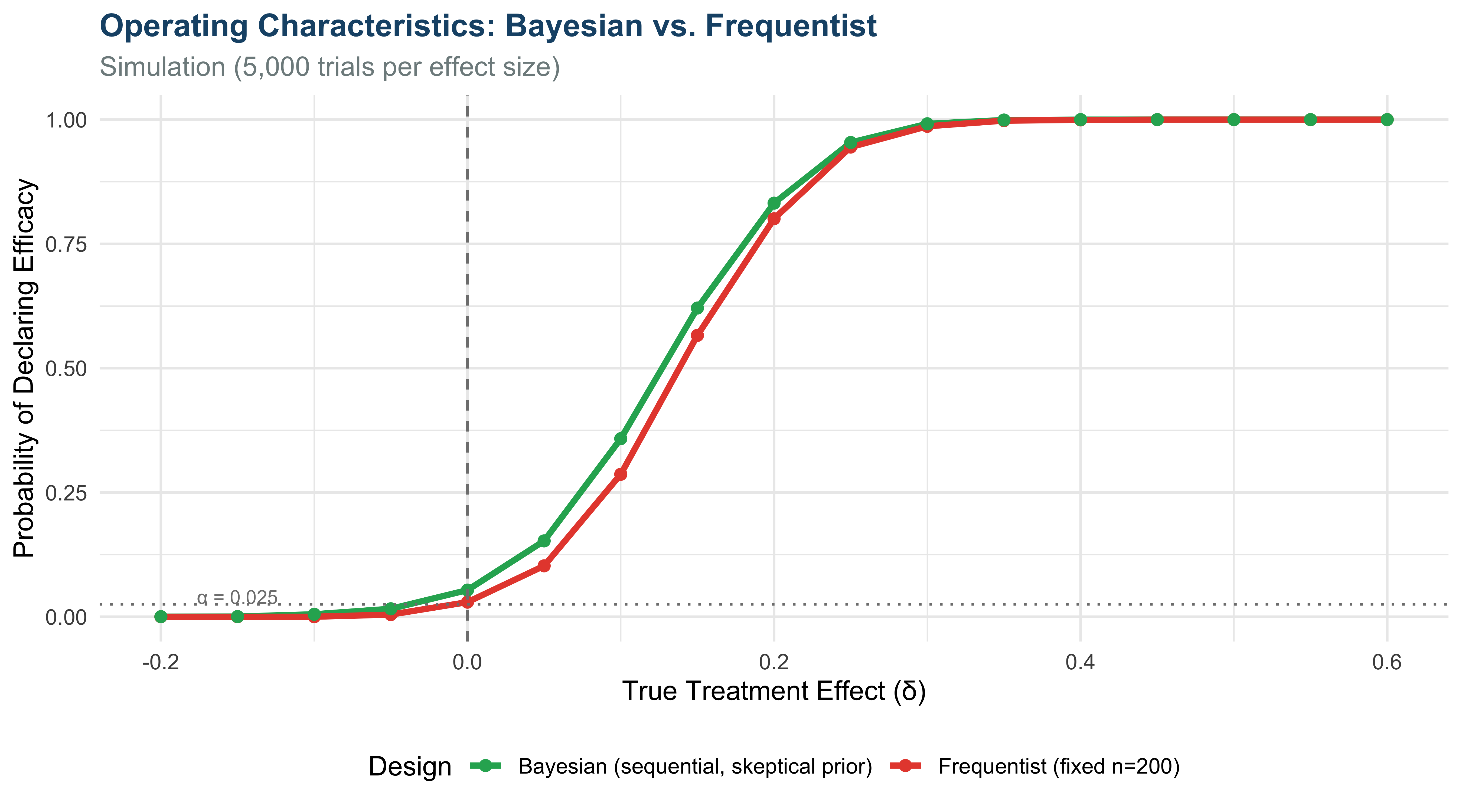
14.2 Simulation: Bayesian vs. Frequentist Operating Characteristics
Show code
library(ggplot2)

set.seed(42)
n_sims <- 5000
true_effects <- seq(-0.2, 0.6, by = 0.05)
n_fixed <- 200 # per arm

results <- data.frame()

for (delta in true_effects) {
  # Frequentist: fixed sample, z-test
  freq_reject <- 0
  for (s in 1:n_sims) {
    y <- rnorm(n_fixed, delta, 1)
    se <- 1 / sqrt(n_fixed)
    z <- mean(y) / se
    if (z > qnorm(0.975)) freq_reject <- freq_reject + 1
  }

  # Bayesian: skeptical prior N(0, 0.35^2), sequential looks every 50 patients
  prior_mean <- 0; prior_sd <- 0.35
  bayes_reject <- 0
  bayes_avg_n <- 0
  for (s in 1:n_sims) {
    all_y <- rnorm(n_fixed, delta, 1)
    stopped <- FALSE
    for (look_n in seq(50, n_fixed, by = 50)) {
      y_cum <- all_y[1:look_n]
      obs_mean <- mean(y_cum)
      obs_se <- 1 / sqrt(look_n)
      post_var <- 1 / (1/prior_sd^2 + 1/obs_se^2)
      post_mean <- post_var * (prior_mean/prior_sd^2 + obs_mean/obs_se^2)
      post_sd <- sqrt(post_var)
      prob_eff <- 1 - pnorm(0, post_mean, post_sd)
      if (prob_eff > 0.975) {
        bayes_reject <- bayes_reject + 1
        bayes_avg_n <- bayes_avg_n + look_n
        stopped <- TRUE
        break
      }
    }
    if (!stopped) bayes_avg_n <- bayes_avg_n + n_fixed
  }

  results <- rbind(results, data.frame(
    delta = rep(delta, 2),
    power = c(freq_reject/n_sims, bayes_reject/n_sims),
    method = c("Frequentist (fixed n=200)", "Bayesian (sequential, skeptical prior)")
  ))
}

ggplot(results, aes(x = delta, y = power, color = method)) +
  geom_line(linewidth = 1.3) +
  geom_point(size = 2) +
  geom_vline(xintercept = 0, linetype = "dashed", color = "grey50") +
  geom_hline(yintercept = 0.025, linetype = "dotted", color = "grey50") +
  annotate("text", x = -0.15, y = 0.04, label = "α = 0.025", size = 3, color = "grey50") +
  scale_color_manual(values = c("Frequentist (fixed n=200)" = "#e74c3c",
                                 "Bayesian (sequential, skeptical prior)" = "#27ae60")) +
  labs(x = "True Treatment Effect (δ)", y = "Probability of Declaring Efficacy",
       title = "Operating Characteristics: Bayesian vs. Frequentist",
       subtitle = paste0("Simulation (", format(n_sims, big.mark=","), " trials per effect size)"),
       color = "Design") +
  theme_minimal(base_size = 12) +
  theme(
    plot.title = element_text(face = "bold", color = "#1a5276", size = 14),
    plot.subtitle = element_text(color = "#7f8c8d"),
    legend.position = "bottom"
  )
14.3 Document Prepared for Blood Cancer Talks
Hosts: Ashwin, Raj Chakraborty, Eddie Cliff
Guest: Frank Harrell, PhD — Professor of Biostatistics, Vanderbilt University
Topic: FDA Guidance on Bayesian Methodology in Clinical Trials
This document integrates the FDA’s 2019 Adaptive Designs Guidance, the 2026 Bayesian Methodology Draft Guidance, Stephen Senn’s “Beware of the Morlocks” critique (March 2026), Frank Harrell’s Statistical Thinking framework, and the uploaded 2019 FDA Adaptive Designs guidance document.
Document generated with Quarto using R R version 4.6.1 (2026-06-24) and Python. All code is reproducible and available via the “Show code” toggles above.